
9.2: Paired Samples for Two Means
- Page ID
- 5214

\( \newcommand{\vecs}[1]{\overset { \scriptstyle \rightharpoonup} {\mathbf{#1}} } \)
\( \newcommand{\vecd}[1]{\overset{-\!-\!\rightharpoonup}{\vphantom{a}\smash {#1}}} \)
\( \newcommand{\id}{\mathrm{id}}\) \( \newcommand{\Span}{\mathrm{span}}\)
( \newcommand{\kernel}{\mathrm{null}\,}\) \( \newcommand{\range}{\mathrm{range}\,}\)
\( \newcommand{\RealPart}{\mathrm{Re}}\) \( \newcommand{\ImaginaryPart}{\mathrm{Im}}\)
\( \newcommand{\Argument}{\mathrm{Arg}}\) \( \newcommand{\norm}[1]{\| #1 \|}\)
\( \newcommand{\inner}[2]{\langle #1, #2 \rangle}\)
\( \newcommand{\Span}{\mathrm{span}}\)
\( \newcommand{\id}{\mathrm{id}}\)
\( \newcommand{\Span}{\mathrm{span}}\)
\( \newcommand{\kernel}{\mathrm{null}\,}\)
\( \newcommand{\range}{\mathrm{range}\,}\)
\( \newcommand{\RealPart}{\mathrm{Re}}\)
\( \newcommand{\ImaginaryPart}{\mathrm{Im}}\)
\( \newcommand{\Argument}{\mathrm{Arg}}\)
\( \newcommand{\norm}[1]{\| #1 \|}\)
\( \newcommand{\inner}[2]{\langle #1, #2 \rangle}\)
\( \newcommand{\Span}{\mathrm{span}}\) \( \newcommand{\AA}{\unicode[.8,0]{x212B}}\)
\( \newcommand{\vectorA}[1]{\vec{#1}} % arrow\)
\( \newcommand{\vectorAt}[1]{\vec{\text{#1}}} % arrow\)
\( \newcommand{\vectorB}[1]{\overset { \scriptstyle \rightharpoonup} {\mathbf{#1}} } \)
\( \newcommand{\vectorC}[1]{\textbf{#1}} \)
\( \newcommand{\vectorD}[1]{\overrightarrow{#1}} \)
\( \newcommand{\vectorDt}[1]{\overrightarrow{\text{#1}}} \)
\( \newcommand{\vectE}[1]{\overset{-\!-\!\rightharpoonup}{\vphantom{a}\smash{\mathbf {#1}}}} \)
\( \newcommand{\vecs}[1]{\overset { \scriptstyle \rightharpoonup} {\mathbf{#1}} } \)
\( \newcommand{\vecd}[1]{\overset{-\!-\!\rightharpoonup}{\vphantom{a}\smash {#1}}} \)
\(\newcommand{\avec}{\mathbf a}\) \(\newcommand{\bvec}{\mathbf b}\) \(\newcommand{\cvec}{\mathbf c}\) \(\newcommand{\dvec}{\mathbf d}\) \(\newcommand{\dtil}{\widetilde{\mathbf d}}\) \(\newcommand{\evec}{\mathbf e}\) \(\newcommand{\fvec}{\mathbf f}\) \(\newcommand{\nvec}{\mathbf n}\) \(\newcommand{\pvec}{\mathbf p}\) \(\newcommand{\qvec}{\mathbf q}\) \(\newcommand{\svec}{\mathbf s}\) \(\newcommand{\tvec}{\mathbf t}\) \(\newcommand{\uvec}{\mathbf u}\) \(\newcommand{\vvec}{\mathbf v}\) \(\newcommand{\wvec}{\mathbf w}\) \(\newcommand{\xvec}{\mathbf x}\) \(\newcommand{\yvec}{\mathbf y}\) \(\newcommand{\zvec}{\mathbf z}\) \(\newcommand{\rvec}{\mathbf r}\) \(\newcommand{\mvec}{\mathbf m}\) \(\newcommand{\zerovec}{\mathbf 0}\) \(\newcommand{\onevec}{\mathbf 1}\) \(\newcommand{\real}{\mathbb R}\) \(\newcommand{\twovec}[2]{\left[\begin{array}{r}#1 \\ #2 \end{array}\right]}\) \(\newcommand{\ctwovec}[2]{\left[\begin{array}{c}#1 \\ #2 \end{array}\right]}\) \(\newcommand{\threevec}[3]{\left[\begin{array}{r}#1 \\ #2 \\ #3 \end{array}\right]}\) \(\newcommand{\cthreevec}[3]{\left[\begin{array}{c}#1 \\ #2 \\ #3 \end{array}\right]}\) \(\newcommand{\fourvec}[4]{\left[\begin{array}{r}#1 \\ #2 \\ #3 \\ #4 \end{array}\right]}\) \(\newcommand{\cfourvec}[4]{\left[\begin{array}{c}#1 \\ #2 \\ #3 \\ #4 \end{array}\right]}\) \(\newcommand{\fivevec}[5]{\left[\begin{array}{r}#1 \\ #2 \\ #3 \\ #4 \\ #5 \\ \end{array}\right]}\) \(\newcommand{\cfivevec}[5]{\left[\begin{array}{c}#1 \\ #2 \\ #3 \\ #4 \\ #5 \\ \end{array}\right]}\) \(\newcommand{\mattwo}[4]{\left[\begin{array}{rr}#1 \amp #2 \\ #3 \amp #4 \\ \end{array}\right]}\) \(\newcommand{\laspan}[1]{\text{Span}\{#1\}}\) \(\newcommand{\bcal}{\cal B}\) \(\newcommand{\ccal}{\cal C}\) \(\newcommand{\scal}{\cal S}\) \(\newcommand{\wcal}{\cal W}\) \(\newcommand{\ecal}{\cal E}\) \(\newcommand{\coords}[2]{\left\{#1\right\}_{#2}}\) \(\newcommand{\gray}[1]{\color{gray}{#1}}\) \(\newcommand{\lgray}[1]{\color{lightgray}{#1}}\) \(\newcommand{\rank}{\operatorname{rank}}\) \(\newcommand{\row}{\text{Row}}\) \(\newcommand{\col}{\text{Col}}\) \(\renewcommand{\row}{\text{Row}}\) \(\newcommand{\nul}{\text{Nul}}\) \(\newcommand{\var}{\text{Var}}\) \(\newcommand{\corr}{\text{corr}}\) \(\newcommand{\len}[1]{\left|#1\right|}\) \(\newcommand{\bbar}{\overline{\bvec}}\) \(\newcommand{\bhat}{\widehat{\bvec}}\) \(\newcommand{\bperp}{\bvec^\perp}\) \(\newcommand{\xhat}{\widehat{\xvec}}\) \(\newcommand{\vhat}{\widehat{\vvec}}\) \(\newcommand{\uhat}{\widehat{\uvec}}\) \(\newcommand{\what}{\widehat{\wvec}}\) \(\newcommand{\Sighat}{\widehat{\Sigma}}\) \(\newcommand{\lt}{<}\) \(\newcommand{\gt}{>}\) \(\newcommand{\amp}{&}\) \(\definecolor{fillinmathshade}{gray}{0.9}\)Are two populations the same? Is the average height of men taller than the average height of women? Is the mean weight less after a diet than before?
You can compare populations by comparing their means. You take a sample from each population and compare the statistics.
Anytime you compare two populations you need to know if the samples are independent or dependent. The formulas you use are different for different types of samples.
If how you choose one sample has no effect on the way you choose the other sample, the two samples are independent. The way to think about it is that in independent samples, the individuals from one sample are overall different from the individuals from the other sample. This will mean that sample one has no affect on sample two. The sample values from one sample are not related or paired with values from the other sample.
If you choose the samples so that a measurement in one sample is paired with a measurement from the other sample, the samples are dependent or matched or paired. (Often a before and after situation.) You want to make sure the there is a meaning for pairing data values from one sample with a specific data value from the other sample. One way to think about it is that in dependent samples, the individuals from one sample are the same individuals from the other sample, though there can be other reasons to pair values. This makes the sample values from each sample paired.
Example \(\PageIndex{1}\) independent or dependent samples
Determine if the following are dependent or independent samples.
- Randomly choose 5 men and 6 women and compare their heights.
- Choose 10 men and weigh them. Give them a new wonder diet drug and later weigh them again.
- Take 10 people and measure the strength of their dominant arm and their non-dominant arm.
Solution
- Independent, since there is no reason that one value belongs to another. The individuals are not the same for both samples. The individuals are definitely different. A way to think about this is that the knowledge that a man is chosen in one sample does not give any information about any of the woman chosen in the other sample.
- Dependent, since each person’s before weight can be matched with their after weight. The individuals are the same for both samples. A way to think about this is that the knowledge that a person weighs 400 pounds at the beginning will tell you something about their weight after the diet drug.
- Dependent, since you can match the two arm strengths. The individuals are the same for both samples. So the knowledge of one person’s dominant arm strength will tell you something about the strength of their non-dominant arm.
To analyze data when there are matched or paired samples, called dependent samples, you conduct a paired t-test. Since the samples are matched, you can find the difference between the values of the two random variables.
Hypothesis Test for Two Sample Paired t-Test
- State the random variables and the parameters in words.
\(x_{1}\) = random variable 1
\(x_{2}\) = random variable 2
\(\mu_{1}\) = mean of random variable 1
\(\mu_{2}\) = mean of random variable 2 - State the null and alternative hypotheses and the level of significance The usual hypotheses would be
\(\begin{array}{ll}{H_{o} : \mu_{1}=\mu_{2} \text { or }} & {H_{o} : \mu_{1}-\mu_{2}=0} \\ {H_{A} : \mu_{1}<\mu_{2}} & {H_{A} : \mu_{1}-\mu_{2}<0} \\ {H_{A} : \mu_{1}>\mu_{2}} & {H_{A} : \mu_{1}-\mu_{2}>0} \\ {H_{A} : \mu_{1} \neq \mu_{2}} & {H_{A} : \mu_{1}-\mu_{2} \neq 0}\end{array}\)
However, since you are finding the differences, then you can actually think of \(\mu_{1}-\mu_{2}=\mu_{\sigma} \mu_{d}=\) population mean value of the differences,
So the hypotheses become
\(\begin{array}{l}{H_{o} : \mu_{d}=0} \\ {H_{1} : \mu_{d}<0} \\ {H_{A} : \mu_{d}>0} \\ {H_{A} : \mu_{d} \neq 0}\end{array}\)
Also, state your \(\alpha\) level here. - State and check the assumptions for the hypothesis test
- A random sample of n pairs is taken.
- The population of the difference between random variables is normally distributed. In this case the population you are interested in has to do with the differences that you find. It does not matter if each random variable is normally distributed. It is only important if the differences you find are normally distributed. Just as before, the t-test is fairly robust to the assumption if the sample size is large. This means that if this assumption isn’t met, but your sample size is quite large (over 30), then the results of the t-test are valid.
- Find the sample statistic, test statistic, and p-value
Sample Statistic:
Difference: \(d=x_{1}-x_{2}\)for each pair
Sample mean of the differences: \(\overline{d}=\dfrac{\sum d}{n}\)
Standard deviation of the differences: \(s_{d}=\dfrac{\sum(d-\overline{d})^{2}}{n-1}\)
Number of pairs: n
Test Statistic:
\(t=\dfrac{\overline{d}-\mu_{d}}{\dfrac{s_{d}}{\sqrt{n}}}\)
with degrees of freedom = df = n - 1p-value:Note
\(\mu_{d}=0\) in most cases.
On TI-83/84: Use tcdf ( lower limit, upper limit, df )On R: Use pt (t, df )Note
If \(H_{A} : \mu_{d}<0\), then lower limit is \(-1 E 99\) and upper limit is your test statistic. If \(H_{A} : \mu_{d}>0\), then lower limit is your test statistic and the upper limit is \(1 E 99\). If \(H_{A} : \mu_{d} \neq 0\), then find the p-value for \(H_{A} : \mu_{d}<0\), and multiply by 2.)
Note
If \(H_{A} : \mu_{d}<0\), use pt (t, df ). If \(H_{A} : \mu_{d}>0\), use 1 - pt(t, df). If \(H_{A} : \mu_{d} \neq 0\), then find the p-value for \(H_{A} : \mu_{d}<0\), and multiply by 2
- This is where you write reject \(H_{o}\) or fail to reject \(H_{o}\). The rule is: if the p-value < \(\alpha\), then reject \(H_{o}\). If the p-value \(\geq \alpha\), then fail to reject \(H_{o}\).
- This is where you interpret in real world terms the conclusion to the test. The conclusion for a hypothesis test is that you either have enough evidence to show \(H_{A}\) is true, or you do not have enough evidence to show \(H_{A}\) is true.
Confidence Interval for Difference in Means from Paired Samples (t-Interval)
The confidence interval for the difference in means has the same random variables and means and the same assumptions as the hypothesis test for two paired samples. If you have already completed the hypothesis test, then you do not need to state them again. If you haven’t completed the hypothesis test, then state the random variables and means, and state and check the assumptions before completing the confidence interval step.
- Find the sample statistic and confidence interval
Sample Statistic:
Difference: d = \(x_{1}-x_{2}\)
Sample mean of the differences: \(\overline{d}=\dfrac{\sum{d}}{n}\)
Standard deviation of the differences: \(s_{d}=\dfrac{\sum(d-\overline{d})^{2}}{n-1}\)
Number of pairs: n
Confidence Interval:
The confidence interval estimate of the difference \(\mu_{d}=\mu_{1}-\mu_{2}\) is
\(\begin{array}{l}{\overline{d}-E<\mu_{d}<\overline{d}+E} \\ {E=t_{c} \dfrac{s_{d}}{\sqrt{n}}}\end{array}\)
\(t_{c}\) is the critical value where degrees of freedom df = n - 1 - Statistical Interpretation: In general this looks like, “there is a C% chance that the statement \(\overline{d}-E<\mu_{d}<\overline{d}+E\) contains the true mean difference.”
- Real World Interpretation: This is where you state what interval contains the true mean difference.
The critical value is a value from the Student’s t-distribution. Since a confidence interval is found by adding and subtracting a margin of error amount from the sample mean, and the interval has a probability of containing the true mean difference, then you can think of this as the statement \(P\left(\overline{d}-E<\mu_{d}<\overline{d}+E\right)=C\). To find the critical value, you use table A.2 in the Appendix.
How to check the assumptions of t-test and confidence interval:
In order for the t-test or confidence interval to be valid, the assumptions of the test must be met. So whenever you run a t-test or confidence interval, you must make sure the assumptions are met. So you need to check them. Here is how you do this:
- For the assumption that the sample is a random sample, describe how you took the samples. Make sure your sampling technique is random and that the samples were dependent.
- For the assumption that the population of the differences is normal, remember the process of assessing normality from chapter 6.
Example \(\PageIndex{2}\) hypothesis test for paired samples using the formula
A researcher wants to see if a weight loss program is effective. She measures the weight of 6 randomly selected women before and after the weight loss program (see Example \(\PageIndex{1}\)). Is there evidence that the weight loss program is effective? Test at the 5% level.
| Person | 1 | 2 | 3 | 4 | 5 | 6 |
| Weight before | 165 | 172 | 181 | 185 | 168 | 175 |
| Weight after | 143 | 151 | 156 | 161 | 152 | 154 |
- State the random variables and the parameters in words.
- State the null and alternative hypotheses and the level of significance.
- State and check the assumptions for the hypothesis test.
- Find the sample statistic, test statistic, and p-value.
- Conclusion
- Interpretation
Solution
1. \(x_{1}\) = weight of a woman after the weight loss program
\(x_{2}\) = weight of a woman before the weight loss program
\(\mu_{1}\) = mean weight of a woman after the weight loss program
\(\mu_{2}\) = mean weight of a woman before the weight loss program
2. \(\begin{array}{l}{H_{o} : \mu_{d}=0} \\ {H_{A} : \mu_{d}<0} \\ {\alpha=0.05}\end{array}\)
3.
- A random sample of 6 pairs of weights before and after was taken. This was stated in the problem, since the women were chosen randomly.
- The population of the difference in after and before weights is normally distributed. To see if this is true, look at the histogram, number of outliers, and the normal probability plot. (If you wish, you can look at the normal probability plot first. If it doesn’t look linear, then you may want to look at the histogram and number of outliers at this point.)
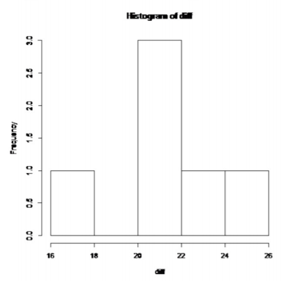.png?revision=1)
This histogram looks somewhat bell shaped.
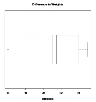.png?revision=1)
There is only one outlier in the difference data set.
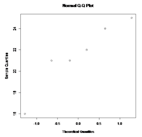.png?revision=1)
The probability plot on the differences looks somewhat linear. So you can assume that the distribution of the difference in weights is normal.
4. Sample Statistics:
| Person | 1 | 2 | 3 | 4 | 5 | 6 |
| Weight after, \(x_{1}\) | 143 | 151 | 156 | 161 | 152 | 154 |
| Weight before, \(x_{2}\) | 165 | 172 | 181 | 185 | 168 | 175 |
| d = \(x_{1}-x_{2}\) | -22 | -21 | -25 | -24 | -16 | -21 |
The mean and standard deviation are
\(\begin{array}{l}{\overline{d}=-21.5} \\ {s_{d}=3.15}\end{array}\)
Test Statistic:
\(t=\dfrac{\overline{d}-\mu_{d}}{s_{d} / \sqrt{n}}=\dfrac{-21.5-0}{3.15 / \sqrt{6}}=-16.779\)
p-value:
There are six pairs so the degrees of freedom are
df = n - 1 = 6 - 1 = 5
Since \(H_{1} : \mu_{d}<0\), then p-value
Using TI-83/84: tcdf \((-1 E 99,-16.779,5) \approx 6.87 \times 10^{-6}\)
Using R: pt \((-16.779,5) \approx 6.87 \times 10^{-6}\)
5. Since the p-value < 0.05, reject \(H_{o}\).
6. There is enough evidence to show that the weight loss program is effective.
Note
Just because the hypothesis test says the program is effective doesn’t mean you should go out and use it right away. The program has statistical significance, but that doesn’t mean it has practical significance. You need to see how much weight a person loses, and you need to look at how safe it is, how expensive, does it work in the long term, and other type questions. Remember to look at the practical significance in all situations. In this case, the average weight loss was 21.5 pounds, which is very practically significant. Do remember to look at the safety and expense of the drug also.
Example \(\PageIndex{3}\) hypothesis Test for Paired Samples Using Technology
The New Zealand Air Force purchased a batch of flight helmets. They then found out that the helmets didn’t fit. In order to make sure that they order the correct size helmets, they measured the head size of recruits. To save money, they wanted to use cardboard calipers, but were not sure if they will be accurate enough. So they took 18 recruits and measured their heads with the cardboard calipers and also with metal calipers. The data in centimeters (cm) is in Example \(\PageIndex{3}\) ("NZ helmet size," 2013). Do the data provide enough evidence to show that there is a difference in measurements between the cardboard and metal calipers? Use a 5% level of significance.
| Cardboard | Metal |
|---|---|
| 146 | 145 |
| 151 | 153 |
| 163 | 161 |
| 152 | 151 |
| 151 | 145 |
| 151 | 150 |
| 149 | 150 |
| 166 | 163 |
| 149 | 147 |
| 155 | 154 |
| 155 | 150 |
| 156 | 156 |
| 162 | 161 |
| 150 | 152 |
| 156 | 154 |
| 158 | 154 |
| 149 | 147 |
| 163 | 160 |
- State the random variables and the parameters in words.
- State the null and alternative hypotheses and the level of significance.
- State and check the assumptions for the hypothesis test.
- Find the sample statistic, test statistic, and p-value.
- Conclusion
- Interpretation
Solution
1. \(x_{1}\) = head measurement of recruit using cardboard caliper
\(x_{2}\) = head measurement of recruit using metal caliper
\(\mu_{1}\) = mean head measurement of recruit using cardboard caliper
\(\mu_{2}\) = mean head measurement of recruit using metal caliper
2. \(\begin{array}{l}{H_{o} : \mu_{d}=0} \\ {H_{A} : \mu_{d} \neq 0} \\ {\alpha=0.05}\end{array}\)
3.
- A random sample of 18 pairs of head measures of recruits with cardboard and metal caliper was taken. This was not stated, but probably could be safely assumed.
- The population of the difference in head measurements between cardboard and metal calipers is normally distributed. To see if this is true, look at the histogram, number of outliers, and the normal probability plot. (If you wish, you can look at the normal probability plot first. If it doesn’t look linear, then you may want to look at the histogram and number of outliers at this point.)
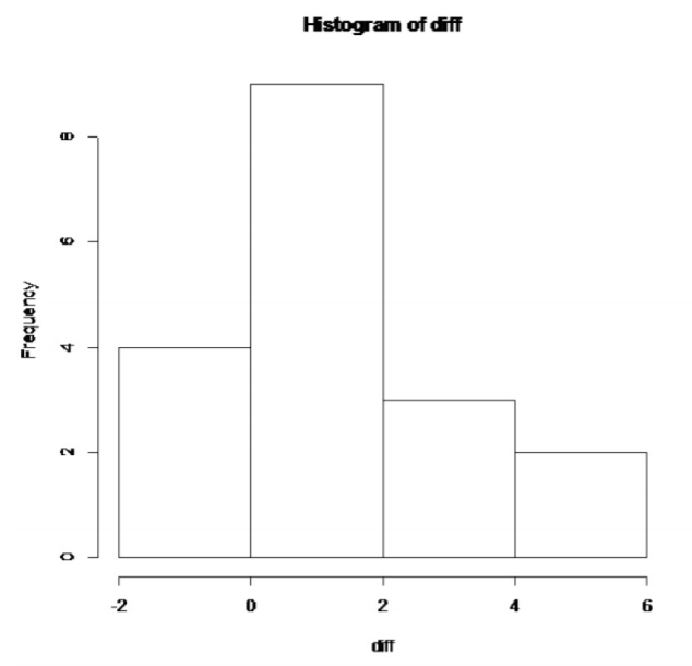.png?revision=1)
This histogram looks bell shaped.
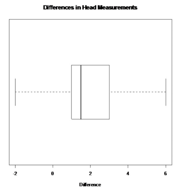.png?revision=1)
There are no outliers in the difference data set.
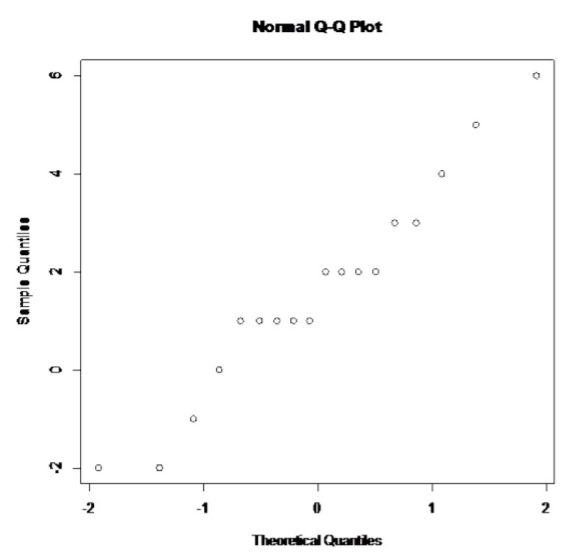.png?revision=1)
The probability plot on the differences looks somewhat linear.
So you can assume that the distribution of the difference in weights is normal.
4. Using the TI-83/84, put \(x_{1}\) into L1 and \(x_{2}\) into L2. Then go onto the name L3, and type L1-L2. The calculator will calculate the differences for you and put them in L3. Now go into STAT and move over to TESTS. Choose T-Test. The setup for the calculator is in Figure \(\PageIndex{7}\).
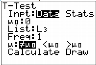.png?revision=1)
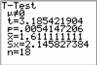
Once you press ENTER on Calculate you will see the result shown in Figure \(\PageIndex{8}\).
.png?revision=1)
Using R: command is t.test(variable1, variable2, paired = TRUE, alternative = "less" or "greater"). For this example, the command would be t.test(cardboard, metal, paired = TRUE)
Paired t-test
data: cardboard and metal
t = 3.1854, df = 17, p-value = 0.005415
alternative hypothesis: true difference in means is not equal to 0
95 percent confidence interval:
0.5440163 2.6782060
sample estimates:
mean of the differences
1.611111
The t = 3.185 is the test statistic. The p-value is 0.0054147206.
5. Since the p-value < 0.05, reject \(H_{o}\).
6. There is enough evidence to show that the mean head measurements using the cardboard calipers are not the same as when using the metal calipers. So it looks like the New Zealand Air Force shouldn’t use the cardboard calipers.
Example \(\PageIndex{4}\) confidence interval for paired samples using the formula
A researcher wants to estimate the mean weight loss that people experience using a new program. She measures the weight of 6 randomly selected women before and after the weight loss program (see Example \(\PageIndex{1}\)). Find a 90% confidence interval for the mean the weight loss using the new program.
- State the random variables and the parameters in words.
- State and check the assumptions for the confidence interval.
- Find the sample statistic and confidence interval.
- Statistical Interpretation
- Real World Interpretation
Solution
1. These were stated in Example \(\PageIndex{2}\), but are reproduced here for reference.
\(x_{1}\) = weight of a woman after the weight loss program
\(x_{2}\) = weight of a woman before the weight loss program
\(\mu_{1}\) = mean weight of a woman after the weight loss program
\(\mu_{2}\) = mean weight of a woman before the weight loss program
2. The assumptions were stated and checked in Example \(\PageIndex{2}\).
3. Sample Statistics:
From Example \(\PageIndex{2}\)
\(\begin{array}{l}{\overline{d}=-21.5} \\ {s_{d}=3.15}\end{array}\)
The confidence level is 90%, so
C= 90%
There are six pairs, so the degrees of freedom are
df = n - 1 = 6 - 1 = 5
Now look in table A.2. Go down the first column to 5, then over to the column headed with 90%.
\(t_{c}=2.015\)
\(E=t_{c} \dfrac{s_{d}}{\sqrt{n}}=2.015 \dfrac{3.15}{\sqrt{6}} \approx 2.6\)
\(\overline{d}-E<\mu_{d}<\overline{d}+E\)
\(-21.5-2.6<\mu_{d}<-21.5+2.6\)
\(-24.1 \text { pounds }<\mu_{d}<-18.9 \text { pounds }\)
4. There is a 90% chance that \(-24.1 \text { pounds }<\mu_{d}<-18.9 \text { pounds }\) contains the true mean difference in weight loss.
5. The mean weight loss is between 18.9 and 24.1 pounds.
Note
The negative signs tell you that the first mean is less than the second mean, and thus a weight loss in this case.
Example \(\PageIndex{5}\) confidence interval for paired samples using technology
The New Zealand Air Force purchased a batch of flight helmets. They then found out that the helmets didn’t fit. In order to make sure that they order the correct size helmets, they measured the head size of recruits. To save money, they wanted to use cardboard calipers, but were not sure if they will be accurate enough. So they took 18 recruits and measured their heads with the cardboard calipers and also with metal calipers. The data in centimeters (cm) is in Example \(\PageIndex{3}\) ("NZ helmet size," 2013). Estimate the mean difference in measurements between the cardboard and metal calipers using a 95% confidence interval.
- State the random variables and the parameters in words.
- State and check the assumptions for the hypothesis test.
- Find the sample statistic and confidence interval.
- Statistical Interpretation
- Real World Interpretation
Solution
1. These were stated in Example \(\PageIndex{3}\), but are reproduced here for reference.
\(x_{1}\) = head measurement of recruit using cardboard caliper
\(x_{2}\) = head measurement of recruit using metal caliper
\(\mu_{1}\) = mean head measurement of recruit using cardboard caliper
\(\mu_{2}\) = mean head measurement of recruit using metal caliper
2. The assumptions were stated and checked in Example \(\PageIndex{3}\).
3. Using the TI-83/84, put \(x_{1}\) into L1 and \(x_{2}\) into L2. Then go onto the name L3, and type L1 - L2. The calculator will now calculate the differences for you and put them in L3. Now go into STAT and move over to TESTS. Then chose TInterval. The setup for the calculator is in Figure \(\PageIndex{9}\).
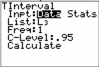.png?revision=1)
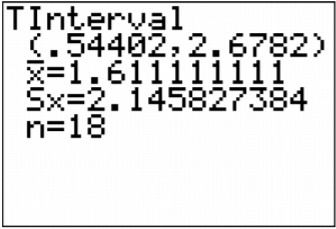
Once you press ENTER on Calculate you will see the result shown in Figure \(\PageIndex{10}\).
.png?revision=1)
Using R: the command is t.test(variable1, variable2, paired = TRUE, conf.level = C), where C is in decimal form. For this example the command would be
t.test(cardboard, metal, paired = TRUE, conf.level=0.95)
Paired t-test
data: cardboard and metal
t = 3.1854, df = 17, p-value = 0.005415
alternative hypothesis: true difference in means is not equal to 0
95 percent confidence interval:
0.5440163 2.6782060
sample estimates:
mean of the differences
1.611111
So
\(0.54 \mathrm{cm}<\mu_{d}<2.68 \mathrm{cm}\)
4. There is a 95% chance that \(0.54 \mathrm{cm}<\mu_{d}<2.68 \mathrm{cm}\) contains the true mean difference in head measurements between cardboard and metal calibers.
5. The mean difference in head measurements between the cardboard and metal calibers is between 0.54 and 2.68 cm. This means that the cardboard calibers measure on average the head of a recruit to be between 0.54 and 2.68 cm more in diameter than the metal calibers. That makes it seem that the cardboard calibers are not measuring the same as the metal calibers. (The positive values on the confidence interval imply that the first mean is higher than the second mean.)
Examples 9.2.2 and 9.2.4 use the same data set, but one is conducting a hypothesis test and the other is conducting a confidence interval. Notice that the hypothesis test’s conclusion was to reject \(H_{o}\) and say that there was a difference in the means, and the confidence interval does not contain the number 0. If the confidence interval did contain the number 0, then that would mean that the two means could be the same. Since the interval did not contain 0, then you could say that the means are different just as in the hypothesis test. This means that the hypothesis test and the confidence interval can produce the same interpretation. Do be careful though, you can run a hypothesis test with a particular significance level and a confidence interval with a confidence level that is not compatible with your significance level. This will mean that the conclusion from the confidence interval would not be the same as with a hypothesis test. So if you want to estimate the mean difference, then conduct a confidence interval. If you want to show that the means are different, then conduct a hypothesis test.
Homework
Exercise \(\PageIndex{1}\)
In each problem show all steps of the hypothesis test or confidence interval. If some of the assumptions are not met, note that the results of the test or interval may not be correct and then continue the process of the hypothesis test or confidence interval.
- The cholesterol level of patients who had heart attacks was measured two days after the heart attack and then again four days after the heart attack. The researchers want to see if the cholesterol level of patients who have heart attacks reduces as the time since their heart attack increases. The data is in Example \(\PageIndex{4}\) ("Cholesterol levels after," 2013). Do the data show that the mean cholesterol level of patients that have had a heart attack reduces as the time increases since their heart attack? Test at the 1% level.
Patient Cholesterol Level Day 2 Cholesterol Level Day 4 1 270 218 2 236 234 3 210 214 4 142 116 5 280 200 6 272 276 7 160 146 8 220 182 9 225 238 10 242 288 11 186 190 12 266 236 13 206 244 14 318 258 15 294 240 16 282 294 17 234 220 18 224 200 19 276 220 20 282 186 21 360 352 22 310 202 23 280 218 24 278 248 25 288 278 26 288 248 27 244 270 28 236 242 Table \(\PageIndex{4}\): Cholesterol Levels in (mg/dL) of Heart Attack Patients - The cholesterol level of patients who had heart attacks was measured two days after the heart attack and then again four days after the heart attack. The researchers want to see if the cholesterol level of patients who have heart attacks reduces as the time since their heart attack increases. The data is in Example \(\PageIndex{4}\) ("Cholesterol levels after," 2013). Calculate a 98% confidence interval for the mean difference in cholesterol levels from day two to day four.
- All Fresh Seafood is a wholesale fish company based on the east coast of the U.S. Catalina Offshore Products is a wholesale fish company based on the west coast of the U.S. Example \(\PageIndex{5}\) contains prices from both companies for specific fish types ("Seafood online," 2013) ("Buy sushi grade," 2013). Do the data provide enough evidence to show that a west coast fish wholesaler is more expensive than an east coast wholesaler? Test at the 5% level.
Fish All Fresh Seafood Prices Catalina Offshore Product Prices Cod 19.99 17.99 Tilapi 6.00 13.99 Farmed Salmon 19.99 22.99 Organic Salmon 24.99 24.99 Grouper Fillet 29.99 19.99 Tuna 28.99 31.99 Swordfish 23.99 23.99 Sea Bass 32.99 23.99 Striped Bass 29.99 14.99 Table \(\PageIndex{5}\): Wholesale Prices of Fish in Dollars - All Fresh Seafood is a wholesale fish company based on the east coast of the U.S. Catalina Offshore Products is a wholesale fish company based on the west coast of the U.S. Example \(\PageIndex{5}\) contains prices from both companies for specific fish types ("Seafood online," 2013) ("Buy sushi grade," 2013). Find a 95% confidence interval for the mean difference in wholesale price between the east coast and west coast suppliers.
- The British Department of Transportation studied to see if people avoid driving on Friday the 13th. They did a traffic count on a Friday and then again on a Friday the 13th at the same two locations ("Friday the 13th," 2013). The data for each location on the two different dates is in Example \(\PageIndex{6}\). Do the data show that on average fewer people drive on Friday the 13th? Test at the 5% level.
Dates 6th 13th 1990, July 139246 138548 1990, July 134012 132909 1991, September 137055 136018 1991, September 133732 131843 1991, December 123552 121641 1991, December 121139 118723 1992, March 128293 125532 1992, March 124631 120249 1992, November 124609 122770 1992, November 117584 117263 Table \(\PageIndex{6}\): Traffic Count - The British Department of Transportation studied to see if people avoid driving on Friday the 13th. They did a traffic count on a Friday and then again on a Friday the 13th at the same two locations ("Friday the 13th," 2013). The data for each location on the two different dates is in Example \(\PageIndex{6}\). Estimate the mean difference in traffic count between the 6th and the 13th using a 90% level.
- To determine if Reiki is an effective method for treating pain, a pilot study was carried out where a certified second-degree Reiki therapist provided treatment on volunteers. Pain was measured using a visual analogue scale (VAS) immediately before and after the Reiki treatment (Olson & Hanson, 1997). The data is in Example \(\PageIndex{7}\). Do the data show that Reiki treatment reduces pain? Test at the 5% level.
VAS before VAS after 6 3 2 1 2 0 9 1 3 0 3 2 4 1 5 2 2 2 3 0 5 1 2 2 3 0 5 1 1 0 6 4 6 1 4 4 4 1 7 6 2 1 4 3 8 8 Table \(\PageIndex{7}\): Pain Measures Before and After Reiki Treatment - To determine if Reiki is an effective method for treating pain, a pilot study was carried out where a certified second-degree Reiki therapist provided treatment on volunteers. Pain was measured using a visual analogue scale (VAS) immediately before and after the Reiki treatment (Olson & Hanson, 1997). The data is in Example \(\PageIndex{7}\). Compute a 90% confidence level for the mean difference in VAS score from before and after Reiki treatment.
- The female labor force participation rates (FLFPR) of women in randomly selected countries in 1990 and latest years of the 1990s are in Example \(\PageIndex{8}\) (Lim, 2002). Do the data show that the mean female labor force participation rate in 1990 is different from that in the latest years of the 1990s using a 5% level of significance?
Region and country FLFPR 25-54 1990 FLFPR 25-54 Latest years of 1990s Iran 22.6 12.5 Morocco 41.4 34.5 Qatar 42.3 46.5 Syrian Arab Republic 25.6 19.5 United Arab Emirates 36.4 39.7 Cape Verde 46.7 50.9 Ghana 89.8 90.0 Kenya 82.1 82.6 Lesotho 51.9 68.0 South Africa 54.7 61.7 Bangladesh 73.5 60.6 Malaysia 49.0 50.2 Mongolia 84.7 71.3 Myanmar 72.1 72.3 Argentina 36.8 54 Belize 28.8 42.5 Bolivia 27.3 69.8 Brazil 51.1 63.2 Colombia 57.4 72.7 Ecuador 33.5 64 Nicaragua 50.1 42.5 Uruguay 59.5 71.5 Albania 77.4 78.8 Uzbekistan 79.6 82.8 Table \(\PageIndex{8}\): Female Labor Force Participation Rates - The female labor force participation rates of women in randomly selected countries in 1990 and latest years of the 1990s are in Example \(\PageIndex{8}\) (Lim, 2002). Estimate the mean difference in the female labor force participation rate in 1990 to latest years of the 1990s using a 95% confidence level?
- Example \(\PageIndex{9}\) contains pulse rates collected from males, who are non-smokers but do drink alcohol ("Pulse rates before," 2013). The before pulse rate is before they exercised, and the after pulse rate was taken after the subject ran in place for one minute. Do the data indicate that the pulse rate before exercise is less than after exercise? Test at the 1% level.
Pulse before Pulse after 76 88 56 110 64 126 50 90 49 83 68 136 68 125 88 150 80 146 78 168 59 92 60 104 65 82 76 150 145 155 84 140 78 141 85 131 78 132 Table \(\PageIndex{9}\): Pulse Rate of Males Before and After Exercise - Example \(\PageIndex{9}\) contains pulse rates collected from males, who are non-smokers but do drink alcohol ("Pulse rates before," 2013). The before pulse rate is before they exercised, and the after pulse rate was taken after the subject ran in place for one minute. Compute a 98% confidence interval for the mean difference in pulse rates from before and after exercise.
- Answer
-
For all hypothesis tests, just the conclusion is given. For all confidence intervals, just the interval using technology is given. See solution for the entire answer.
1. Reject Ho
2. \(5.39857 \mathrm{mg} / \mathrm{dL}<\mu_{d}<41.1729 \mathrm{mg} / \mathrm{dL}\)
3. Fail to reject Ho
4. \(-\$ 3.24216<\mu_{d}<\$ 8.13327\)
5. Reject Ho
6. \(1154.09<\mu_{d}<2517.51\)
7. Reject Ho
8. \(1.499<\mu_{d}<3.001\)
9. Fail to reject Ho
10. \(-10.9096 \%<\mu_{d}<0.2596 \%\)
11. Reject Ho
12. \(-62.0438 \text { beats/min }<\mu_{d}<-37.1141 \text { beats/min }\)