
5.1: Basics of Probability Distributions
- Page ID
- 5185

\( \newcommand{\vecs}[1]{\overset { \scriptstyle \rightharpoonup} {\mathbf{#1}} } \)
\( \newcommand{\vecd}[1]{\overset{-\!-\!\rightharpoonup}{\vphantom{a}\smash {#1}}} \)
\( \newcommand{\id}{\mathrm{id}}\) \( \newcommand{\Span}{\mathrm{span}}\)
( \newcommand{\kernel}{\mathrm{null}\,}\) \( \newcommand{\range}{\mathrm{range}\,}\)
\( \newcommand{\RealPart}{\mathrm{Re}}\) \( \newcommand{\ImaginaryPart}{\mathrm{Im}}\)
\( \newcommand{\Argument}{\mathrm{Arg}}\) \( \newcommand{\norm}[1]{\| #1 \|}\)
\( \newcommand{\inner}[2]{\langle #1, #2 \rangle}\)
\( \newcommand{\Span}{\mathrm{span}}\)
\( \newcommand{\id}{\mathrm{id}}\)
\( \newcommand{\Span}{\mathrm{span}}\)
\( \newcommand{\kernel}{\mathrm{null}\,}\)
\( \newcommand{\range}{\mathrm{range}\,}\)
\( \newcommand{\RealPart}{\mathrm{Re}}\)
\( \newcommand{\ImaginaryPart}{\mathrm{Im}}\)
\( \newcommand{\Argument}{\mathrm{Arg}}\)
\( \newcommand{\norm}[1]{\| #1 \|}\)
\( \newcommand{\inner}[2]{\langle #1, #2 \rangle}\)
\( \newcommand{\Span}{\mathrm{span}}\) \( \newcommand{\AA}{\unicode[.8,0]{x212B}}\)
\( \newcommand{\vectorA}[1]{\vec{#1}} % arrow\)
\( \newcommand{\vectorAt}[1]{\vec{\text{#1}}} % arrow\)
\( \newcommand{\vectorB}[1]{\overset { \scriptstyle \rightharpoonup} {\mathbf{#1}} } \)
\( \newcommand{\vectorC}[1]{\textbf{#1}} \)
\( \newcommand{\vectorD}[1]{\overrightarrow{#1}} \)
\( \newcommand{\vectorDt}[1]{\overrightarrow{\text{#1}}} \)
\( \newcommand{\vectE}[1]{\overset{-\!-\!\rightharpoonup}{\vphantom{a}\smash{\mathbf {#1}}}} \)
\( \newcommand{\vecs}[1]{\overset { \scriptstyle \rightharpoonup} {\mathbf{#1}} } \)
\( \newcommand{\vecd}[1]{\overset{-\!-\!\rightharpoonup}{\vphantom{a}\smash {#1}}} \)
\(\newcommand{\avec}{\mathbf a}\) \(\newcommand{\bvec}{\mathbf b}\) \(\newcommand{\cvec}{\mathbf c}\) \(\newcommand{\dvec}{\mathbf d}\) \(\newcommand{\dtil}{\widetilde{\mathbf d}}\) \(\newcommand{\evec}{\mathbf e}\) \(\newcommand{\fvec}{\mathbf f}\) \(\newcommand{\nvec}{\mathbf n}\) \(\newcommand{\pvec}{\mathbf p}\) \(\newcommand{\qvec}{\mathbf q}\) \(\newcommand{\svec}{\mathbf s}\) \(\newcommand{\tvec}{\mathbf t}\) \(\newcommand{\uvec}{\mathbf u}\) \(\newcommand{\vvec}{\mathbf v}\) \(\newcommand{\wvec}{\mathbf w}\) \(\newcommand{\xvec}{\mathbf x}\) \(\newcommand{\yvec}{\mathbf y}\) \(\newcommand{\zvec}{\mathbf z}\) \(\newcommand{\rvec}{\mathbf r}\) \(\newcommand{\mvec}{\mathbf m}\) \(\newcommand{\zerovec}{\mathbf 0}\) \(\newcommand{\onevec}{\mathbf 1}\) \(\newcommand{\real}{\mathbb R}\) \(\newcommand{\twovec}[2]{\left[\begin{array}{r}#1 \\ #2 \end{array}\right]}\) \(\newcommand{\ctwovec}[2]{\left[\begin{array}{c}#1 \\ #2 \end{array}\right]}\) \(\newcommand{\threevec}[3]{\left[\begin{array}{r}#1 \\ #2 \\ #3 \end{array}\right]}\) \(\newcommand{\cthreevec}[3]{\left[\begin{array}{c}#1 \\ #2 \\ #3 \end{array}\right]}\) \(\newcommand{\fourvec}[4]{\left[\begin{array}{r}#1 \\ #2 \\ #3 \\ #4 \end{array}\right]}\) \(\newcommand{\cfourvec}[4]{\left[\begin{array}{c}#1 \\ #2 \\ #3 \\ #4 \end{array}\right]}\) \(\newcommand{\fivevec}[5]{\left[\begin{array}{r}#1 \\ #2 \\ #3 \\ #4 \\ #5 \\ \end{array}\right]}\) \(\newcommand{\cfivevec}[5]{\left[\begin{array}{c}#1 \\ #2 \\ #3 \\ #4 \\ #5 \\ \end{array}\right]}\) \(\newcommand{\mattwo}[4]{\left[\begin{array}{rr}#1 \amp #2 \\ #3 \amp #4 \\ \end{array}\right]}\) \(\newcommand{\laspan}[1]{\text{Span}\{#1\}}\) \(\newcommand{\bcal}{\cal B}\) \(\newcommand{\ccal}{\cal C}\) \(\newcommand{\scal}{\cal S}\) \(\newcommand{\wcal}{\cal W}\) \(\newcommand{\ecal}{\cal E}\) \(\newcommand{\coords}[2]{\left\{#1\right\}_{#2}}\) \(\newcommand{\gray}[1]{\color{gray}{#1}}\) \(\newcommand{\lgray}[1]{\color{lightgray}{#1}}\) \(\newcommand{\rank}{\operatorname{rank}}\) \(\newcommand{\row}{\text{Row}}\) \(\newcommand{\col}{\text{Col}}\) \(\renewcommand{\row}{\text{Row}}\) \(\newcommand{\nul}{\text{Nul}}\) \(\newcommand{\var}{\text{Var}}\) \(\newcommand{\corr}{\text{corr}}\) \(\newcommand{\len}[1]{\left|#1\right|}\) \(\newcommand{\bbar}{\overline{\bvec}}\) \(\newcommand{\bhat}{\widehat{\bvec}}\) \(\newcommand{\bperp}{\bvec^\perp}\) \(\newcommand{\xhat}{\widehat{\xvec}}\) \(\newcommand{\vhat}{\widehat{\vvec}}\) \(\newcommand{\uhat}{\widehat{\uvec}}\) \(\newcommand{\what}{\widehat{\wvec}}\) \(\newcommand{\Sighat}{\widehat{\Sigma}}\) \(\newcommand{\lt}{<}\) \(\newcommand{\gt}{>}\) \(\newcommand{\amp}{&}\) \(\definecolor{fillinmathshade}{gray}{0.9}\)As a reminder, a variable or what will be called the random variable from now on, is represented by the letter x and it represents a quantitative (numerical) variable that is measured or observed in an experiment.
Also remember there are different types of quantitative variables, called discrete or continuous. What is the difference between discrete and continuous data? Discrete data can only take on particular values in a range. Continuous data can take on any value in a range. Discrete data usually arises from counting while continuous data usually arises from measuring.
Examples of each
How tall is a plant given a new fertilizer? Continuous. This is something you measure. How many fleas are on prairie dogs in a colony? Discrete. This is something you count.
If you have a variable, and can find a probability associated with that variable, it is called a random variable. In many cases the random variable is what you are measuring, but when it comes to discrete random variables, it is usually what you are counting. So for the example of how tall is a plant given a new fertilizer, the random variable is the height of the plant given a new fertilizer. For the example of how many fleas are on prairie dogs in a colony, the random variable is the number of fleas on a prairie dog in a colony.
Now suppose you put all the values of the random variable together with the probability that that random variable would occur. You could then have a distribution like before, but now it is called a probability distribution since it involves probabilities. A probability distribution is an assignment of probabilities to the values of the random variable. The abbreviation of pdf is used for a probability distribution function.
For probability distributions, \(0 \leq P(x) \leq 1 \operatorname{and} \sum P(x)=1\)
Example \(\PageIndex{1}\): Probability Distribution
The 2010 U.S. Census found the chance of a household being a certain size. The data is in Example \(\PageIndex{1}\) ("Households by age," 2013).
| Size of household | 1 | 2 | 3 | 4 | 5 | 6 | 7 or more |
| Probability | 26.7% | 33.6% | 15.8% | 13.7% | 6.3% | 2.4% | 1.5% |
Solution
In this case, the random variable is x = number of people in a household. This is a discrete random variable, since you are counting the number of people in a household.
This is a probability distribution since you have the x value and the probabilities that go with it, all of the probabilities are between zero and one, and the sum of all of the probabilities is one.
You can give a probability distribution in table form (as in Example \(\PageIndex{1}\)) or as a graph. The graph looks like a histogram. A probability distribution is basically a relative frequency distribution based on a very large sample.
Example \(\PageIndex{2}\) graphing a probability distribution
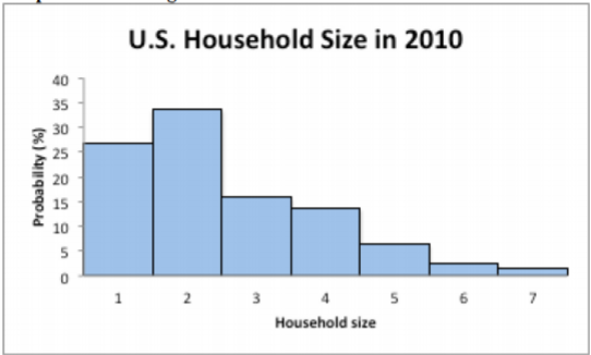
The 2010 U.S. Census found the chance of a household being a certain size. The data is in the table ("Households by age," 2013). Draw a histogram of the probability distribution.
| Size of household | 1 | 2 | 3 | 4 | 5 | 6 | 7 or more |
| Probability | 26.7% | 33.6% | 15.8% | 13.7% | 6.3% | 2.4% | 1.5% |
Solution
State random variable:
x = number of people in a household
You draw a histogram, where the x values are on the horizontal axis and are the x values of the classes (for the 7 or more category, just call it 7). The probabilities are on the vertical axis.
.png?revision=1)
Notice this graph is skewed right.
Just as with any data set, you can calculate the mean and standard deviation. In problems involving a probability distribution function (pdf), you consider the probability distribution the population even though the pdf in most cases come from repeating an experiment many times. This is because you are using the data from repeated experiments to estimate the true probability. Since a pdf is basically a population, the mean and standard deviation that are calculated are actually the population parameters and not the sample statistics. The notation used is the same as the notation for population mean and population standard deviation that was used in chapter 3.
Note
The mean can be thought of as the expected value. It is the value you expect to get if the trials were repeated infinite number of times. The mean or expected value does not need to be a whole number, even if the possible values of x are whole numbers.
For a discrete probability distribution function,
The mean or expected value is \(\mu=\sum x P(x)\)
The variance is \(\sigma^{2}=\sum(x-\mu)^{2} P(x)\)
The standard deviation is \(\sigma=\sqrt{\sum(x-\mu)^{2} P(x)}\)
where x = the value of the random variable and P(x) = the probability corresponding to a particular x value.
Example \(\PageIndex{3}\): Calculating mean, variance, and standard deviation for a discrete probability distribution
The 2010 U.S. Census found the chance of a household being a certain size. The data is in the table ("Households by age," 2013).
| Size of household | 1 | 2 | 3 | 4 | 5 | 6 | 7 or more |
| Probability | 26.7% | 33.6% | 15.8% | 13.7% | 6.3% | 2.4% | 1.5% |
- Find the mean
- Find the variance
- Find the standard deviation
- Use a TI-83/84 to calculate the mean and standard deviation
- Using R to calculate the mean
Solution
State random variable:
x= number of people in a household
a. To find the mean it is easier to just use a table as shown below. Consider the category 7 or more to just be 7. The formula for the mean says to multiply the x value by the P(x) value, so add a row into the table for this calculation. Also convert all P(x) to decimal form.
| x | 1 | 2 | 3 | 4 | 5 | 6 | 7 |
| P(x) | 0.267 | 0.336 | 0.158 | 0.137 | 0.063 | 0.024 | 0.015 |
| xP(x) | 0.267 | 0.672 | 0.474 | 0.548 | 0.315 | 0.144 | 0.098 |
Now add up the new row and you get the answer 2.525. This is the mean or the expected value, \(\mu\) = 2.525 people. This means that you expect a household in the U.S. to have 2.525 people in it. Now of course you can’t have half a person, but what this tells you is that you expect a household to have either 2 or 3 people, with a little more 3-person households than 2-person households.
b. To find the variance, again it is easier to use a table version than try to just the formula in a line. Looking at the formula, you will notice that the first operation that you should do is to subtract the mean from each x value. Then you square each of these values. Then you multiply each of these answers by the probability of each x value. Finally you add up all of these values.
| x | 1 | 2 | 3 | 4 | 5 | 6 | 7 |
| P(x) | 0.267 | 0.336 | 0.158 | 0.137 | 0.063 | 0.024 | 0.015 |
| \(x-\mu\) | -1.525 | -0.525 | 0.475 | 1.475 | 2.475 | 3.475 | 4.475 |
| \((x-\mu)^{2}\) | 2.3256 | 0.2756 | 0.2256 | 2.1756 | 6.1256 | 12.0756 | 20.0256 |
| \((x-\mu)^{2} P(x)\) | 0.6209 | 0.0926 | 0.0356 | 0.2981 | 0.3859 | 0.2898 | 0.3004 |
Now add up the last row to find the variance, \(\sigma^{2}=2.02375 \text { people }^{2}\). (Note: try not to round your numbers too much so you aren’t creating rounding error in your answer. The numbers in the table above were rounded off because of space limitations, but the answer was calculated using many decimal places.)
c. To find the standard deviation, just take the square root of the variance, \(\sigma=\sqrt{2.023375} \approx 1.422454\) people. This means that you can expect a U.S. household to have 2.525 people in it, with a standard deviation of 1.42 people.
d. Go into the STAT menu, then the Edit menu. Type the x values into L1 and the P(x) values into L2. Then go into the STAT menu, then the CALC menu. Choose 1:1-Var Stats. This will put 1-Var Stats on the home screen. Now type in L1,L2 (there is a comma between L1 and L2) and then press ENTER. If you have the newer operating system on the TI-84, then your input will be slightly different. You will see the output in Figure \(\PageIndex{1}\).
.png?revision=1)
The mean is 2.525 people and the standard deviation is 1.422 people.
e. The command would be weighted.mean(x, p). So for this example, the process would look like:
x<-c(1, 2, 3, 4, 5, 6, 7)
p<-c(0.267, 0.336, 0.158, 0.137, 0.063, 0.024, 0.015)
weighted.mean(x, p)
Output:
[1] 2.525
So the mean is 2.525.
To find the standard deviation, you would need to program the process into R. So it is easier to just do it using the formula.
Example \(\PageIndex{4}\) Calculating the expected value
In the Arizona lottery called Pick 3, a player pays $1 and then picks a three-digit number. If those three numbers are picked in that specific order the person wins $500. What is the expected value in this game?
Solution
To find the expected value, you need to first create the probability distribution. In this case, the random variable x = winnings. If you pick the right numbers in the right order, then you win $500, but you paid $1 to play, so you actually win $499. If you didn’t pick the right numbers, you lose the $1, the x value is -$1. You also need the probability of winning and losing. Since you are picking a three-digit number, and for each digit there are 10 numbers you can pick with each independent of the others, you can use the multiplication rule. To win, you have to pick the right numbers in the right order. The first digit, you pick 1 number out of 10, the second digit you pick 1 number out of 10, and the third digit you pick 1 number out of 10. The probability of picking the right number in the right order is \(\dfrac{1}{10} * \dfrac{1}{10} * \dfrac{1}{10}=\dfrac{1}{1000}=0.001\). The probability of losing (not winning) would be \(1-\dfrac{1}{1000}=\dfrac{999}{1000}=0.999\). Putting this information into a table will help to calculate the expected value.
| Win or lose | x | P(x) | xP(x) |
| Win | $499 | 0.001 | $0.499 |
| Lose | -$1 | 0.999 | -$0.999 |
Now add the two values together and you have the expected value. It is \(\$ 0.499+(-\$ 0.999)=-\$ 0.50\). In the long run, you will expect to lose $0.50. Since the expected value is not 0, then this game is not fair. Since you lose money, Arizona makes money, which is why they have the lottery.
The reason probability is studied in statistics is to help in making decisions in inferential statistics. To understand how that is done the concept of a rare event is needed.
Definition \(\PageIndex{1}\): Rare Event Rule for Inferential Statistics
If, under a given assumption, the probability of a particular observed event is extremely small, then you can conclude that the assumption is probably not correct.
An example of this is suppose you roll an assumed fair die 1000 times and get a six 600 times, when you should have only rolled a six around 160 times, then you should believe that your assumption about it being a fair die is untrue.
Determining if an event is unusual
If you are looking at a value of x for a discrete variable, and the P(the variable has a value of x or more) < 0.05, then you can consider the x an unusually high value. Another way to think of this is if the probability of getting such a high value is less than 0.05, then the event of getting the value x is unusual.
Similarly, if the P(the variable has a value of x or less) < 0.05, then you can consider this an unusually low value. Another way to think of this is if the probability of getting a value as small as x is less than 0.05, then the event x is considered unusual.
Why is it "x or more" or "x or less" instead of just "x" when you are determining if an event is unusual? Consider this example: you and your friend go out to lunch every day. Instead of Going Dutch (each paying for their own lunch), you decide to flip a coin, and the loser pays for both. Your friend seems to be winning more often than you'd expect, so you want to determine if this is unusual before you decide to change how you pay for lunch (or accuse your friend of cheating). The process for how to calculate these probabilities will be presented in the next section on the binomial distribution. If your friend won 6 out of 10 lunches, the probability of that happening turns out to be about 20.5%, not unusual. The probability of winning 6 or more is about 37.7%. But what happens if your friend won 501 out of 1,000 lunches? That doesn't seem so unlikely! The probability of winning 501 or more lunches is about 47.8%, and that is consistent with your hunch that this isn't so unusual. But the probability of winning exactly 501 lunches is much less, only about 2.5%. That is why the probability of getting exactly that value is not the right question to ask: you should ask the probability of getting that value or more (or that value or less on the other side).
The value 0.05 will be explained later, and it is not the only value you can use.
Example \(\PageIndex{5}\) is the event unusual
The 2010 U.S. Census found the chance of a household being a certain size. The data is in the table ("Households by age," 2013).
| Size of household | 1 | 2 | 3 | 4 | 5 | 6 | 7 or more |
| Probability | 26.7% | 33.6% | 15.8% | 13.7% | 6.3% | 2.4% | 1.5% |
- Is it unusual for a household to have six people in the family?
- If you did come upon many families that had six people in the family, what would you think?
- Is it unusual for a household to have four people in the family?
- If you did come upon a family that has four people in it, what would you think?
Solution
State random variable:
x= number of people in a household
a. To determine this, you need to look at probabilities. However, you cannot just look at the probability of six people. You need to look at the probability of x being six or more people or the probability of x being six or less people. The
\(\begin{aligned} P(x \leq 6) &=P(x=1)+P(x=2)+P(x=3)+P(x=4)+P(x=5)+P(x=6) \\ &=26.7 \%+33.6 \%+15.8 \%+13.7 \%+6.3 \%+2.4 \% \\ &=98.5 \% \end{aligned}\)
Since this probability is more than 5%, then six is not an unusually low value. The
\(\begin{aligned} P(x \geq 6) &=P(x=6)+P(x \geq 7) \\ &=2.4 \%+1.5 \% \\ &=3.9 \% \end{aligned}\)
Since this probability is less than 5%, then six is an unusually high value. It is unusual for a household to have six people in the family.
b. Since it is unusual for a family to have six people in it, then you may think that either the size of families is increasing from what it was or that you are in a location where families are larger than in other locations.
c. To determine this, you need to look at probabilities. Again, look at the probability of x being four or more or the probability of x being four or less. The
\(\begin{aligned} P(x \geq 4) &=P(x=4)+P(x=5)+P(x=6)+P(x=7) \\ &=13.7 \%+6.3 \%+2.4 \%+1.5 \% \\ &=23.9 \% \end{aligned}\)
Since this probability is more than 5%, four is not an unusually high value. The
\(\begin{aligned} P(x \leq 4) &=P(x=1)+P(x=2)+P(x=3)+P(x=4) \\ &=26.7 \%+33.6 \%+15.8 \%+13.7 \% \\ &=89.8 \% \end{aligned}\)
Since this probability is more than 5%, four is not an unusually low value. Thus, four is not an unusual size of a family.
d. Since it is not unusual for a family to have four members, then you would not think anything is amiss.
Homework
Exercise \(\PageIndex{1}\)
- Eyeglassomatic manufactures eyeglasses for different retailers. The number of days it takes to fix defects in an eyeglass and the probability that it will take that number of days are in the table.
Number of days Probabilities 1 24.9% 2 10.8% 3 9.1% 4 12.3% 5 13.3% 6 11.4% 7 7.0% 8 4.6% 9 1.9% 10 1.3% 11 1.0% 12 0.8% 13 0.6% 14 0.4% 15 0.2% 16 0.2% 17 0.1% 18 0.1% Table \(\PageIndex{8}\): Number of Days to Fix Defects
a. State the random variable.
b. Draw a histogram of the number of days to fix defects
c. Find the mean number of days to fix defects.
d. Find the variance for the number of days to fix defects.
e. Find the standard deviation for the number of days to fix defects.
f. Find probability that a lens will take at least 16 days to make a fix the defect.
g. Is it unusual for a lens to take 16 days to fix a defect?
h. If it does take 16 days for eyeglasses to be repaired, what would you think? - Suppose you have an experiment where you flip a coin three times. You then count the number of heads.
- State the random variable.
- Write the probability distribution for the number of heads.
- Draw a histogram for the number of heads.
- Find the mean number of heads.
- Find the variance for the number of heads.
- Find the standard deviation for the number of heads.
- Find the probability of having two or more number of heads.
- Is it unusual for to flip two heads?
- The Ohio lottery has a game called Pick 4 where a player pays $1 and picks a four-digit number. If the four numbers come up in the order you picked, then you win $2,500. What is your expected value?
- An LG Dishwasher, which costs $800, has a 20% chance of needing to be replaced in the first 2 years of purchase. A two-year extended warrantee costs $112.10 on a dishwasher. What is the expected value of the extended warranty assuming it is replaced in the first 2 years?
- Answer
-
1. a. See solutions, b. See solutions, c. 4.175 days, d. 8.414375 \(\text { days }^{2}\), e. 2.901 days, f. 0.004, g. See solutions, h. See solutions
3. -$0.75