4.1: Prelude to p Values

You’ve already seen that \(p\) values are hard to interpret. Getting a statistically insignificant result doesn’t mean there’s no difference. What about getting a significant result?

Let’s try an example. Suppose I am testing a hundred potential cancer medications. Only ten of these drugs actually work, but I don’t know which; I must perform experiments to find them. In these experiments, I’ll look for \(p<0.05\) gains over a placebo, demonstrating that the drug has a significant benefit.

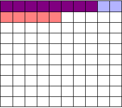
To illustrate, each square in this grid represents one drug. The blue squares are the drugs that work:

Figure \(\PageIndex{1}\)

As we saw, most trials can’t perfectly detect every good medication. We’ll assume my tests have a statistical power of \(0.8\). Of the ten good drugs, I will correctly detect around eight of them, shown in purple:

Figure \(\PageIndex{2}\)

Of the ninety ineffectual drugs, I will conclude that about \(5\) have significant effects. Why? Remember that \(p\) values are calculated under the assumption of no effect, so \(p=0.05\) means a \(5\)% chance of falsely concluding that an ineffectual drug works.

So I perform my experiments and conclude there are \(13\) working drugs: \(8\) good drugs and \(5\) I’ve included erroneously, shown in red:

Figure \(\PageIndex{3}\)

The chance of any given “working” drug being truly effectual is only \(62\)%. If I were to randomly select a drug out of the lot of \(100\), run it through my tests, and discover a \(p<0.05\) statistically significant benefit, there is only a \(62\)% chance that the drug is actually effective. In statistical terms, my false discovery rate – the fraction of statistically significant results which are really false positives – is \(38\)%.

Because the base rate of effective cancer drugs is so low – only \(10\)% of our hundred trial drugs actually work – most of the tested drugs do not work, and we have many opportunities for false positives. If I had the bad fortune of possessing a truckload of completely ineffective medicines, giving a base rate of \(0\)%, there is a \(0\)% chance that any statistically significant result is true. Nevertheless, I will get a \(p<0.05\) result for \(5\)% of the drugs in the truck.

You often hear people quoting \(p\) values as a sign that error is unlikely. “There’s only a \(1\) in \(10,000\) chance this result arose as a statistical fluke,” they say, because they got \(p=0.0001\). No! This ignores the base rate, and is called the base rate fallacy. Remember how \(p\) values are defined:

The P value is defined as the probability, under the assumption of no effect or no difference (the null hypothesis), of obtaining a result equal to or more extreme than what was actually observed.

A \(p\) value is calculated under the assumption that the medication does not work and tells us the probability of obtaining the data we did, or data more extreme than it. It does not tell us the chance the medication is effective.

When someone uses their \(p\) values to say they’re probably right, remember this. Their study’s probability of error is almost certainly much higher. In fields where most tested hypotheses are false, like early drug trials (most early drugs don’t make it through trials), it’s likely that most “statistically significant” results with \(p<0.05\) are actually flukes.

One good example is medical diagnostic tests.