8.6: Using SPSS

As reviewed in Chapter 2, software such as SPSS can be used to expedite analyses once data have been properly entered into the program. Data need to be organized and entered into SPSS in ways that serve the analysis to be conducted. Thus, this section focuses on how to enter and analyze data for an independent samples t-test using SPSS. SPSS version 29 was used for this book; if you are using a different version, you may see some variation from what is shown here.

Entering Data

The independent samples t-tests is bivariate. One variable is used to organize data into comparison groups. The other variable is being compared between those two groups. The variable being compared must be quantitative and should have been measured using numbers on an interval or ratio scale. If these things are all true of your data, you are ready to open SPSS and begin entering your data.

Open the SPSS software, click “New Dataset,” then click “Open” (or “OK” depending on which is shown in the version of the software you are using). This will create a new blank spreadsheet into which you can enter data. There are two tabs which appear towards the bottom of the spreadsheet. One is called “Variable View” which is the tab that allows you to tell the software about your variables. The other is called “Data View” which is the tab that allows you to enter your data.

Click on the Variable View tab. This tab of the spreadsheet has several columns to organize information about the variables. The first column is titled “Name.” Start here and follow these steps:

1. Click the first cell of that column and enter the name of your grouping variable using no spaces, special characters, or symbols. You can name this variable “Group” for simplicity. Hit enter and SPSS will automatically fill in the other cells of that row with some default assumptions about the data.
2. Click the first cell of the column titled “Type” and then click the three dots that appear in the right side of the cell. Specify that the data for that variable appear as numbers by selecting “Numeric.” For numeric data SPSS will automatically allow you to enter values that are up to 8 digits in length with decimals shown to the hundredths place as noted in the “Width” and “Decimal” column headers, respectively. You can edit these as needed to fit your data, though these settings will be appropriate for most variables in the behavioral sciences.
3. Click the first cell of the column titled “Label.” This is where you can specify what you want the variable to be called in output, including in tables and graphs. You can use spaces or phrases here, as desired. For example, you could clarify here that the variable Group refers to “School Groups” by stating as such in the label column for this variable.
4. Click on the three dots in the first cell of the column titled “Values.” This is where you can add details about each group. Click the plus sign and specify that the value 1 (for Group 1) refers to the High School subsample. Then click the plus sign again and specify that value 2 (for Group 2) refers to the College subsample as shown below. Then click “OK.”

5. Click on the first cell of the column titled “Measure.” A pulldown menu with three options will allow you to specify the scale of measurement for the variable. Select the “Nominal.” option because grouping variables are nominal. Now SPSS is set-up for data for the grouping variable.
6. Next we need to set up space for the quantitative variable, starting with the cell under “Name,” enter the name of your quantitative variable using no spaces, special characters, or symbols. You can name this variable “Sleep” for simplicity. Hit enter and SPSS will automatically fill in the other cells of that row with some default assumptions about the data.
7. Click the cell of the column titled “Label.” You can use spaces or phrases here, as desired. For example, you could clarify here that the variable Sleep refers to “Hours of Sleep” by stating as such in the label column for this variable.
8. Click the cell of the column titled “Type” and then click the three dots that appear in the right side of the cell. Specify that the data for that variable appear as numbers by selecting “Numeric.” Again, you can edit the width and decimals as needed to fit your data.
9. Click on the cell of the column titled “Measure.” A pulldown menu with three options will allow you to specify the scale of measurement for the variable. SPSS does not differentiate between interval and ratio and, instead, refers to both of these as “Scale.” Select the “Scale” option because if you are using an independent samples t-test your data for this variable should have been measured on the interval or ratio scale.

Here is what the Variable View tab would look like when created for Data Set 8.1:

Now you are ready to enter your data. Click on the Data View tab toward the bottom of the spreadsheet. This tab of the spreadsheet has several columns into which you can enter the data for each variable. Each column will show the names given to the variables that were entered previously using the Variable View tab. Click the first cell corresponding to the first row of the first column. Start here and follow these steps:

1. Enter the data for the grouping variable moving down the rows under the first column. Put a 1 for in this column for everyone who is a member of Group 1 and put a 2 for this column for everyone who is a member of Group 2.
2. Enter the data for the quantitative variable moving down the rows under the second column. If your data are already on your computer in a spreadsheet format such as excel, you can copy-paste the data in for the variable. Take special care to ensure the Sleep data for Group 1 appear in the rows corresponding to Group 1 and that the Sleep data for Group 2 appear in the rows corresponding to Group 2 as shown below. 3. Then hit save to ensure your data set will be available for you in the future.

Once all the variables have been specified and the data have been entered, you can begin analyzing the data using SPSS.

Conducting an Independent Samples t-Test in SPSS

The steps to running an independent sample t-test in SPSS are:

1. Click Analyze › Compare Means and Proportions › Independent-Samples T Test from the pull down menus as shown below.

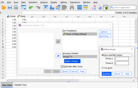
2. Drag the name of the quantitative variable from the list on the left into the Test Variable(s) box on the right of the command window. You can also do this by clicking on the variable name to highlight it and the clicking the arrow to move the variable from the left into the Variable text box on the right. Next, put the grouping variable into the box bearing that name on the right side of the command window. You will need to specify what each group is named so SPSS can group the data accordingly. To do so, click the box that says “Define Groups” under the Grouping Variable section. Indicate that the Groups 1 and 2 are indicated with the numbers “1” and “2”, respectively, as shown below. Then click “Continue” on the Define Groups pop-out window. If the version of SPSS you are using has a check box to estimate effect sizes (as shown in the picture below), click that as well.

3. Click OK.
4. The output (which means the page of calculated results) will appear in a new window of SPSS known as an output viewer. The results will appear in three tables as shown below.

Group Statistics

	School Group	N	Mean	Std. Deviation	Std. Error Mean
Hours of Sleep	High School	5	7.0000	1.58114	.70711
	College	5	5.0000	1.58114	.70711

Independent Samples Test

		Levene's Test for Equality of Variances		t-test for Equality of Means
Hours of Sleep		F	Sig.	t	df	Significance				95% Confidence Interval of the Difference
						One Sided p	Two Sided p	Mean Difference	Std. Error Difference	Lower	Upper
	Equal variances assumed	.000	1.000	2.000	8	.040	.081	2.00000	1.00000	-.30600	4.30600
	Equal variances not assumed			2.000	8.000.	.040	.081	2.00000	1.00000	-.30600	4.30600

Independent Samples Effect Sizes

				95% Confidence Interval
		Standardizer^a	Point Estimate	Lower	Upper
Hours of Sleep	Cohen's d	1.58114	1.2649	-.147	2.615
	Hedges' correction	1.75156	1.1418	-.133	2.361
	Glass's delta	1.58114	1.2649	-.285	2.716

* "a": The denominator used in estimating the effect sizes. Cohen's d uses the pooled standard deviation. Hedges' correction uses the pooled standard deviation, plus a correction factor. Glass's delta uses the sample standard deviation of the control group.

Reading SPSS Output for an Independent Samples t-Test

The first table shows the descriptive statistics for the test. These include the sample size, the sample mean, the sample standard deviation, and the standard error for each group. These are versions of the six foundational pieces that would appear in the formula steps as we saw when we performed hand-calculations for Data Set 8.1 earlier in this chapter. The difference is that the table shows standard deviation whereas the formula uses variance. This is because SPSS is focusing on what you would need to interpret and report results.

The second table shows both one of the assumptions checks and the main test results which are needed for the evidence string, including the t-value, the degrees of freedom (df) and the p value for a one-tailed test (called “One-Sided p” in SPSS) and for a two-tailed test (called a Two Sided p in SPSS).

Let’s start with the assumption check in the second table. The assumptions that must be met to use the standard form of the independent samples t-test is that the variances of the two groups are similar. The Levene’s test for equality of variances is a homogeneity test. When variances are homogeneous enough to meet this assumption, the Levene’s test will have a non-significant p-value (meaning that the two group variance are not significantly uneven). In the output we see the Levene’s test has an obtained F-value of .000 and a “Sig.” value (which is what SPSS calls the p-value) of 1.00. This p-value is greater than .05 indicating that the two group variances are not significantly uneven. This is desirable as it indicates that we have met the assumption of homogeneity of variances and can proceed to reading our results for the t-test.

The second output table shows two versions of the t-test results; those on the top row are for when the assumption of homogeneity is met and those on the bottom are for when this assumption is not met and an adjustment was employed. Our data met this assumption, so we shall use the results shown in the top row. Note: You may notice that the results for the two rows are the same for Data Set 8.1. This is because there was no impact due to unequal variances and, thus, the adjustment was not needed so it had no discernable impact.

We see that the t-value was 2.00, the df was 8, and the p-value was 0.04 for the one-tailed test which means the result was significant. Remember, when using the standard alpha level of .05, a p-value that is less than .05 is significant. These values and conclusion that the result was significant are consistent with what we found when using hand-calculations and comparing the obtained t-value to the critical value that fit our hypothesis and data. Therefore, the results and conclusions when using hand-calculations and when reading the results of SPSS agree. This is what will always happen unless a mistake was made in either the use of hand-calculations or in using SPSS. Note: You will sometimes see slight variation in results due to rounding error when comparing hand-calculated results to SPSS generated results. However, these differences should usually only appear in the third (thousandths) or fourth (ten-thousandths) decimal place; your hand-calculated results will usually match the SPSS generated results to the hundredths place (meaning they should match to two decimal places).

The last table of results in the SPSS output shows the effect sizes. This will only appear if you checked the box in the command window to select this extra analysis. By default, SPSS will provide three calculations of effect size: Cohen’s d, Hedge’s correction, and Glass’s delta. When assumptions of the independent samples t-test are met and total samples sizes are sufficient, Cohen’s d can be used. However, when total sample size is lower than 10, Hedge’s g is preferable. The effect size is reported in the SPSS output table in the column labelled “point estimate.” SPSS reports Cohen’s d in this column as 1.2649, or 1.26 when rounded to the hundredths place for the purposes of reporting in APA format. If you compare the result for Cohen’s d shown in the SPSS output table to our hand-calculations for earlier, you will see they are the same. You may notice that the two estimates of effect size (Cohen’s vs. Hedge’s) differ due to the correction used in Hedge’s but are both considered large.

Choosing and Effect Size

SPSS provides three estimates of effect size, each of which is a better fit for certain scenarios. The default is to use Cohen’s d unless small total sample size or a violation to the assumption of homogeneity of variances warrants a correction. In these cases, use of Hedge’s g or Glass’s delta are recommended, respectively.

• Cohen’s d is appropriate when all assumptions are met and sample sizes are of sufficient size (such as when N = 20 or more).
• Hedge’s g is a corrected version of Cohen’s d which better accounts for small sample sizes. Generally, when total sample size is less than 10, Hedge’s g is more appropriate than Cohen’s d. When the sample size is between 10 and 20, it may be advisable to check both to see how similar or dissimilar they are.
• Glass’s delta is appropriate when group variances are not homogeneous.

Reading Review 8.4

1. What scale of measurement should be indicated in SPSS for the grouping variable?
2. What scale of measurement should be indicated in SPSS for the test variable?
3. What information is used in the output to check that the assumption of homogeneity of variances is met?
4. Under which table and column of the SPSS output can the t-value be found?
5. Under which table and column of the SPSS output can the p-value be found?
6. Under which table and column of the SPSS output can the d-value be found?