5.4: Finding Probabilities

Estimating Sampling Probabilities with the Normal Distribution

As we have just reviewed, the areas under the curve can be used to represent and calculate the proportion of scores in those areas. This also represents the probability that any given score is in that location. Let’s consider this in relation to random sampling. When we randomly sample a score, it means each individual score has an equal chance of being selected. This would mean scores that occur more frequently and which are closer to the peak of the curve are more likely to be randomly selected because there are more of them.

Finding Probabilities using z-Scores

Once a z-score is known, it can be used to calculate probabilities within the normal distribution. This is because the percentages corresponding to areas under the curve represent the probabilities of scores at the corresponding sections of the curve. To say it another way, the percentage of an area in the normal curve is equal to the probability of scores existing and being randomly selected from that area. For example, half of the scores in the normal distribution are expected to be below the mean while the other half are expected to be above it because the mean is the center of the symmetrical normal curve. This also means that the probability that any score selected at random is below the mean is 50% and that the probability that any score selected at random is above the mean is also 50%.

However, not all areas of the curve are as simple to calculate as the two halves. When finding the areas and their corresponding probabilities under the curve, this three step process is useful: 1. Sketch, 2. Shade, and 3. Solve. Start by sketching the normal curve to provide a visual representation of the problem. Next, identify the z-score or z-scores needed and create a vertical line extending up from the z-score(s) location(s) on the x-axis. Shade the area you are solving for. Take note of whether the shaded area includes or extends to the mean and/or includes or extends to one of the tails. 3. Use the z-distribution table to find the percent represented in the shaded region of the sketch. This percentage is equal to the probability of any random score being selected from that area. This three step process can be used to find probabilities below, above, and between z-scores and to compare those probabilities.

Reading the z-Distribution Table

The z-score table, also known as a unit normal table, is located in Appendix C. Here is an excerpt of the z-score table:

Z-Score	Proportion in the Body	Proportion in the Tail	Proportion between the Mean and the Z
0.00	0.5000	0.5000	0.0000
0.01	0.5040	0.4960	0.0040
0.02	0.5080	0.4920	0.0080
0.03	0.5120	0.4880	0.0120
0.04	0.5160	0.4840	0.0160
0.05	0.5199	0.4801	0.0199
0.06	0.5239	0.4761	0.0239
0.07	0.5279	0.4721	0.0279
0.08	0.5319	0.4681	0.0319
0.09	0.5359	0.4641	0.0359
0.10	0.5398	0.4602	0.0398

The z-distribution table shows the areas within the normal curve that are created when a z score is used to divide the graph into segments. Each z-score appears in the first column and the portions it divides the graph into are provided in columns 2 through 4 in decimal form. To convert from decimals to percentages, the proportion must be multiplied by 100. Note that the graph is symmetrical so the absolute values of z-scores are used in column 1 of the z distribution table which allows the table to be used with positive or negative z-scores. However, we must be clear on what each column represents before we can use the table to find proportions of the normal curve:

• Column 2 represents the area from the z-score to its furthest tail. Thus, if a z-score is positive, this is the area from that z-score all the way through the negative tail. If a z score is negative, this is the area from that z-score all the way through the positive tail.
• Column 3 represents the area from a z-score to its nearest tail. For positive z-scores this is the area from the score through the positive tail and for negative z-scores this is the area from the score through the negative tail.
• Column 4 represents the area from a given z-score to the mean (which is at the very center of the graph). For positive z-scores this is the area that goes toward the left from the score until it reaches the center of the curve. For negative z-scores this is the area that goes toward the right from the score until it reaches the center of the curve.

Let’s consider a z-score of 0 (or 0.00 when shown to the hundredths place). We know that this is the center of the curve so the area from it to either tail is 50.00%. The tails are equidistant from the mean so columns 2 (area to the furthest tail) and 3 (area to the closest tail) are both .5000 (which corresponds to 50.00%). There are no scores between a z-score of 0.00 and the mean and, thus, column 4 shows that .0000 (or 0.00%) of score are between a z-score of 0.00 and the mean.

We have briefly reviewed how to read and understand the z-distribution table here but this concept can be complex and used in many different ways. Therefore, we will review seven different ways proportions of the normal curve can be divided and estimated using the z distribution table in detail in the following sections.

Finding Probabilities Below z-Scores

Using Negative z-Scores. The area below a negative z-score will always be less than 50.00%. This is because the whole area below the mean is only 50.00% so any portion of that area must be less than 50.00%. Let’s take a look at an example using the three step process. Suppose you are asked to find the probability that a score below z = -1.50 will be randomly selected. First, sketch the normal curve. Second, draw a vertical line over the location of z = -1.50. Shade the area to the left of that line because lower scores are to the left on the x-axis. This shaded region represents the proportion of the scores that are below a z-score of -1.50 (See Figure 3a). Notice that the shaded area is a small portion of the graph. This is a visual indication that the percentage corresponding to the area will also be small. The shaded area goes from the z-score to the nearest tail so this is the region we need to look up in the z-score table.

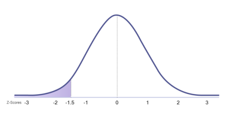
Figure 3a.

We can use the z-distribution table to find the area that corresponds to the area from z = -1.50 to the tail. Remember, the z-distribution table shows the absolute value of each z-score because the normal curve is symmetrical. Therefore, the area from -1.50 to its nearest tail (which is the tail on the left) and from 1.50 to its nearest tail (which is the tail on the right) are the same. Because of this, we can look up the area from 1.50 to the nearest tail in the table and use it to represent the area from -1.50 to its nearest tail. This area is 0.0668 in decimal form or 6.68% when reported as a percentage. Therefore, the probability of a score being randomly selected from below the z-score of -1.50 is 6.68% (See Figure 3b).

Z-Score	Proportion in the Body	Proportion in the Tail	Proportion between the Mean and the Z
1.49	0.9319	0.0681	0.4319
1.50	0.9332	0.0668	0.4332
1.51	0.9345	0.0655	0.4345
1.52	0.9357	0.0643	0.4357
1.53	0.9370	0.0630	0.4370
1.49	0.9319	0.0681	0.4319
0.55	0.7088	0.2912	0.2088

Figure 3a with Proportion Shown.

Using Positive z-Scores. The area below a positive z-score will always be more than 50.00%. This is because the area will start to the right of the mean and extend all the way to the left, subsuming the entire lower half (50.00%) of the graph. Let’s take a look at an example using the three step process. Suppose you are asked to find the probability that a score below z = 1.50 will be randomly selected. First, sketch the normal curve. Second, draw a vertical line over the location of z = 1.50. Shade the area to the left of that line because lower scores are to the left on the x-axis; the shaded region goes to and past the mean all the way into the negative (lower) tail of the graph. This shaded region represents the proportion of the scores that are below a z score of 1.50 (See Figure 4). Notice that the shaded area is a large portion of the graph. This is a visual indication that the percentage corresponding to the area will also be large.

Figure 4.

We already know the area below the mean is 50.00% but need to find the area from z = 1.50 to the mean to get the total area shaded. We can use the z-distribution table to find the area that corresponds to the area from z = 1.50 to the mean. This area is 0.4332 in decimal form or 43.32% when reported as a percentage. We can add this to the 50.00% that is below the mean to get the following: 43.32% + 50.00% = 93.32%. Alternatively, we could look up column 2 of the z-distribution table as it shows the area from a z-score to its furthest mean (which is what we need here). As expected, we see this is also 93.32%. Therefore, the probability of a score being randomly selected from below the z-score of 1.50 is 93.32%.

Z-Score	Proportion in the Body	Proportion in the Tail	Proportion between the Mean and the Z
1.49	0.9319	0.0681	0.4319
1.50	0.9332	0.0668	0.4332
1.51	0.9345	0.0655	0.4345
1.52	0.9357	0.0643	0.4357
1.53	0.9370	0.0630	0.4370
1.49	0.9319	0.0681	0.4319
0.55	0.7088	0.2912	0.2088

Finding Probabilities Above z-Scores

Using Positive z-Scores. The area above a positive z-score will always be less than 50.00%. This is because the whole area above the mean is only 50.00% so any portion of that area must be less than 50.00%. Notice that this the same logic applied to areas below a negative z-score. Suppose you are asked to find the probability that a score above z = 1.50 will be randomly selected. First, sketch the normal curve. Second, draw a vertical line over the location of z = 1.50. Shade the area to the right of that line because higher scores are to the right on the x-axis. This shaded region represents the proportion of the scores that are above a z-score of 1.50 (See Figure 5). Notice that the shaded area is a small portion of the graph. This is a visual indication that the percentage corresponding to the area will also be small. The area shaded goes from the z-score to the tail so this is the region we need to look up in the z-score table.

Figure 5.

We can use the z-distribution table to find the area that corresponds to the area from z = 1.50 to the nearest (right or upper) tail. This area is 0.0668 in decimal form or 6.68% when reported as a percentage. Therefore, the probability of a score being randomly selected from above the z-score of 1.50 is 6.68%. This is the same as the probability of an area below a z-score of -1.50 because the graph is symmetrical and these represent areas which mirror each other in the normal curve.

Using Negative z-Scores. The area above a negative z-score will always be more than 50.00%. This is because the area will start to the right of the mean and extend all the way to the left, subsuming the entire lower half (50.00%) of the graph. Notice that this is the same logic applied to areas below positive z-scores. Let’s take a look at an example using the three step process. Suppose you are asked to find the probability that a score above z = -1.50 will be randomly selected. First, sketch the normal curve. Second, draw a vertical line over the location of z = -1.50. Shade the area to the right of that line because higher scores are to the right on the x axis; the shaded region goes to and past the mean all the way into the positive (upper) tail of the graph. This shaded region represents the proportion of the scores that are above a z-score of -1.50 (See Figure 6). Notice that the shaded area is a large portion of the graph. This is a visual indication that the percentage corresponding to the area will also be large.

Figure 6.

We have two options for finding the shaded region. We already know the area above the mean is 50.00% but need to find the area from z = -1.50 to the mean to get the total area shaded. We can use the z-distribution table to find the area that corresponds to the area from z = -1.50 to the mean (Remember, the z-distribution table shows absolute values of z so we still need the row that corresponds to z = 1.50). This area is 0.4332 in decimal form or 43.32% when reported as a percentage. We can add this to the 50.00% that is above the mean to get the following: 43.32% + 50.00% = 93.32% Therefore, the probability of a score being randomly selected from above the z-score of -1.50 is 93.32%. Alternatively, we can use column 2 of the table which shows the area from the z-score to the furthest tail. Alternatively, we could look up column 2 of the z-distribution table as it shows the area from a z-score to its furthest mean (which is what we need here). As expected, we see this is also 93.32%. The two methods provide the same result so either can be used. Notice that the area above z -1.50 is the same as the probability of an area below a z-score of 1.50 because the graph is symmetrical and these represent areas which mirror each other in the normal curve.

Finding Probabilities Between z-Scores

Finding area between two z-scores is a little more complicated and depends on the direction of the two scores in relation to each other. In order to find the area or probability of a score being randomly selected from between two z-scores, you must first identify whether the two z-scores have opposing signs (meaning one is positive and one is negative) or whether both have the same sign (meaning either both are positive or both are negative). Then, we follow the three step process of sketching, shading, and solving.

Using a Negative and a Positive z-Score. Suppose we want to find the area (or probability of randomly selecting a score) between z = -0.50 and z = 0.75. First, sketch the normal curve. Second, draw a vertical line over the location of z = -0.50 and another over the location of z = 0.75. Shade the area between the two vertical lines. This shaded region represents the proportion of the scores that are between the two z-scores (see Figure 7).

Figure 7.

Keep in mind that the z-distribution table does not tell us area between two z-scores; instead it tells us the areas from each z-score to the mean and to the nearest tail. Notice, however, that the mean is between the two z-scores and is, thus, within the shaded region. This means that the area we are solving for is actually the area from each of the z-scores to the mean added together. Therefore, for step 3 of the process, we must find the area from each z-score to the mean and then add them to get the total for the shaded area. The area from z = -0.50 to the mean is 0.1915 in decimal form or 19.15% when reported as a percentage (see Appendix C for the full z-distribution tables). The area from z = 0.75 to the mean is 0.2734 in decimal form or 27.34% when reported as a percentage. We can add these two areas together to get the total for the shaded area as follows: 19.15% + 27.34% = 46.49% Therefore, the probability of a score being randomly selected from between z-scores of -0.50 and 0.75 is 46.49%.

Using Two Positive z-Scores

To find the area between two positive z-scores, we must find an area that goes neither to the mean nor to the tail so it is a bit unique. Let’s illustrate this with an example. Suppose we want to find the area (or probability of randomly selecting a score) between z = 0.50 and z = 0.75. Start our three step by process by first sketching the normal curve. Second, draw a vertical line over the location of z = 0.50 and another over the location of z = 0.75. Shade the area between the two vertical lines. This shaded region represents the proportion of the scores that are between the two z-scores (see Figure 8a).

Figure 8a.

The z-distribution table will not show us this exact region so we have to get creative to solve for the area in step 3 of the process. Start by finding the area from z = 0.75 to the mean; this area is 0.2734 in decimal form or 27.34% when reported as a percentage. However, we don’t want this total area. Instead, we only want the portion of this area that ends at z = 0.50. Therefore, we want to remove (subtract) the area that goes past 0.50 and to the mean so we will be left with only the shaded region. To do this, we must next find the area from z = 0. 50 to the mean which is 0.1915 in decimal form or 19.15% when reported as a percentage. Finally, we must subtract the smaller area from z = 0.50 to the mean from the larger area of z = 0.75 to the mean to find the shaded area as follows: 27.34% - 19.15% = 8.19% Therefore, the probability of a score being randomly selected from between z-scores of 0.75 and 0.50 is 8.19% (see Figure 8b).

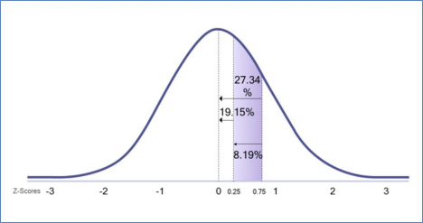
Figure 8b.

Using Two Negative z-Scores

Finding the area between two negative z-scores requires the same logic and process as was used to find the area between two positive z-scores. Let’s illustrate this by using the negative version of the prior example. Suppose we want to find the area (or probability of randomly selecting a score) between z = -0.50 and z = -0.75. Start the three step by process by first sketching the normal curve. Second, draw a vertical line over the location of z = -0.50 and another over the location of z = -0.75. Shade the area between the two vertical lines. This shaded region represents the proportion of the scores that are between the two z-scores (see Figure 9).

Next, find the area from z = -0.75 to the mean; this area is 0.2734 in decimal form or 27.34% when reported as a percentage. However, just as we saw when looking for the area between two positive z-scores, we don’t want this total area. Instead, we only want the portion of this area that ends at z = -0.50. Therefore, we want to remove (subtract) the area that goes from - 0.50 to the mean so we will be left with only the shaded region. To do this, we must next find the area from z = -0. 50 to the mean which is 0.1915 in decimal form or 19.15% when reported as a percentage. Finally, we must subtract the smaller area of z = -0.50 to the mean from the larger area of z = -0.75 to the mean to find the shaded area as follows: 27.34% - 19.15% = 8.19% Therefore, the probability of a score being randomly selected from between z-scores of -0.75 and -0.50 is 8.19%. Notice that this is the same result we got in the prior section when using z = 0.50 and z = 0.75 because the symmetrical nature of the graph causes the left half of the graph to mirror the right half of the graph.

Comparing Probabilities using z-Scores

Comparisons of probabilities can be made using z-scores in a variety of scenarios. First, you can deduce which of two z-scores is more frequently occurring (or more probable) by determining which is closest to z = 0. For example, z = 0.50 is more probable than z = 1.00 because 0.50 is closer to 0 than is 1.00. Second, you can determine which raw scores are most probable by using their z-scores and following the logic in the prior example (i.e. whichever has a z-score closer to 0 is the more probable score). Third, you can compare probabilities of scores being selected from different areas under the curve. For example, we can determine whether there is a greater probability of selecting a z-score between z = 1.00 and z = 2.00 than selecting a z score between z = 2.00 and z = 3.00. It is tempting to focus on the fact that the distance from 1.00 and 2.00 on the x-axis is the same as the distance between 2.00 and 3.00 on the x-axis; this temptation can lead us to erroneously conclude that the probabilities of scores in these two ranges are equal. However, the normal curve slopes and probability is about area in these ranges, not simply distance on the x-axis. If we follow the steps for finding area between z scores, we will find that the area between z-scores of 1.00 and 2.00 is 13.59% and that area between z-scores of 2.00 and 3.00 is 2.15%. This means the probabilities of selecting scores in the aforementioned ranges are 13.59% and 2.15%, respectively. Thus, the probability of randomly selecting a z-score between 1.00 and 2.00 is about six times as high as the probability of randomly selecting a z-score between 2.00 and 3.00.

Finding Percentiles with z-Scores

z-scores can be used to determine percentiles. Percentiles indicate the proportion of scores or cases that are below a given score (see the sections on Percentile Rank Distributions in Chapter 2 to review how percentiles are calculated). For example, if we say someone’s IQ is in the 67% percentile, it means that their IQ is higher than 67% of the scores in the population and that their IQ is lower than 33% of the scores in the population. The total area to the left of a z-score in the normal curve is equivalent to that z score’s percentile. This is because when we solve for area below (left of) a score, we are identifying the proportion of scores lower than it; this is equivalent to the score’s percentile. Thus, there is no special computation or step needed to find percentiles using z-scores. Instead, we simply follow the process for finding area below a z-score. The difference is how we language (or report) the results. When solving for area below a z-score of 0.00, for example, we could report probability or percentile as follows:

Probability: The probability of randomly selecting a score below z = 0.00 is 50%

Percentile: A z-score of 0.00 is at the fiftieth percentile.

Though percentiles are often reported to the whole number for simplicity, it is possible to compute them with more specificity such as by rounding to the hundredths place, just as we have done with z-scores in this chapter.

Finding Raw Scores from Percentiles

Because of the relationships between z-score and percentiles, percentiles can be used to find raw scores if the mean and standard deviation are also known. Suppose you know that the mean IQ score is 100.00 with a standard deviation of 15.00 and are told an individual was in the 67% percentile for IQ. If you wanted to find their raw score, you would follow these steps:

1. Find the z-score that corresponds to the 67th percentile. Note: this is going to be a positive z-score because the percentile is over 50%.
2. Plug that z-score, the mean, and the standard deviation into the z-score formula.
3. Solve for X to find the raw score.

In the example above, we would find the following.

1. The z-score corresponding to the 67th percentile is 0.44 (as shown in the segment of the z-distribution table).

Z-Score	Proportion in the Body	Proportion in the Tail	Proportion between the Mean and the Z
0.43	0.6664	0.3336	0.1664
0.44	0.6700	0.3300	0.1700
0.45	0.6736	0.3264	0.1736

2. Plug z = 0.44, \(\mu\) = 100.00 and \(\sigma\) = 15.00 into the formula \(z=\dfrac{x-\mu}{\sigma}\)as follows: \[0.44=\frac{x-100.00}{15.00} \nonumber \]
3. Solve for x as follows: \[\begin{aligned}
   & 0.44=\frac{x-100.00}{15.00} \\
   & 0.44(15.00)=\frac{x-100.00}{15.00}(15.00) \\
   & 6.60=x-100.00 \\
   & 6.60+100.00=x-100.00+100.00 \\
   & 106.60=x
   \end{aligned} \nonumber \]

This result can be reported as follows:

Summary: An IQ score of 106.60 is in the 67th percentile.