7.5: Inference for Linear Regression
- Page ID
- 315
\( \newcommand{\vecs}[1]{\overset { \scriptstyle \rightharpoonup} {\mathbf{#1}} } \)
\( \newcommand{\vecd}[1]{\overset{-\!-\!\rightharpoonup}{\vphantom{a}\smash {#1}}} \)
\( \newcommand{\dsum}{\displaystyle\sum\limits} \)
\( \newcommand{\dint}{\displaystyle\int\limits} \)
\( \newcommand{\dlim}{\displaystyle\lim\limits} \)
\( \newcommand{\id}{\mathrm{id}}\) \( \newcommand{\Span}{\mathrm{span}}\)
( \newcommand{\kernel}{\mathrm{null}\,}\) \( \newcommand{\range}{\mathrm{range}\,}\)
\( \newcommand{\RealPart}{\mathrm{Re}}\) \( \newcommand{\ImaginaryPart}{\mathrm{Im}}\)
\( \newcommand{\Argument}{\mathrm{Arg}}\) \( \newcommand{\norm}[1]{\| #1 \|}\)
\( \newcommand{\inner}[2]{\langle #1, #2 \rangle}\)
\( \newcommand{\Span}{\mathrm{span}}\)
\( \newcommand{\id}{\mathrm{id}}\)
\( \newcommand{\Span}{\mathrm{span}}\)
\( \newcommand{\kernel}{\mathrm{null}\,}\)
\( \newcommand{\range}{\mathrm{range}\,}\)
\( \newcommand{\RealPart}{\mathrm{Re}}\)
\( \newcommand{\ImaginaryPart}{\mathrm{Im}}\)
\( \newcommand{\Argument}{\mathrm{Arg}}\)
\( \newcommand{\norm}[1]{\| #1 \|}\)
\( \newcommand{\inner}[2]{\langle #1, #2 \rangle}\)
\( \newcommand{\Span}{\mathrm{span}}\) \( \newcommand{\AA}{\unicode[.8,0]{x212B}}\)
\( \newcommand{\vectorA}[1]{\vec{#1}} % arrow\)
\( \newcommand{\vectorAt}[1]{\vec{\text{#1}}} % arrow\)
\( \newcommand{\vectorB}[1]{\overset { \scriptstyle \rightharpoonup} {\mathbf{#1}} } \)
\( \newcommand{\vectorC}[1]{\textbf{#1}} \)
\( \newcommand{\vectorD}[1]{\overrightarrow{#1}} \)
\( \newcommand{\vectorDt}[1]{\overrightarrow{\text{#1}}} \)
\( \newcommand{\vectE}[1]{\overset{-\!-\!\rightharpoonup}{\vphantom{a}\smash{\mathbf {#1}}}} \)
\( \newcommand{\vecs}[1]{\overset { \scriptstyle \rightharpoonup} {\mathbf{#1}} } \)
\(\newcommand{\longvect}{\overrightarrow}\)
\( \newcommand{\vecd}[1]{\overset{-\!-\!\rightharpoonup}{\vphantom{a}\smash {#1}}} \)
\(\newcommand{\avec}{\mathbf a}\) \(\newcommand{\bvec}{\mathbf b}\) \(\newcommand{\cvec}{\mathbf c}\) \(\newcommand{\dvec}{\mathbf d}\) \(\newcommand{\dtil}{\widetilde{\mathbf d}}\) \(\newcommand{\evec}{\mathbf e}\) \(\newcommand{\fvec}{\mathbf f}\) \(\newcommand{\nvec}{\mathbf n}\) \(\newcommand{\pvec}{\mathbf p}\) \(\newcommand{\qvec}{\mathbf q}\) \(\newcommand{\svec}{\mathbf s}\) \(\newcommand{\tvec}{\mathbf t}\) \(\newcommand{\uvec}{\mathbf u}\) \(\newcommand{\vvec}{\mathbf v}\) \(\newcommand{\wvec}{\mathbf w}\) \(\newcommand{\xvec}{\mathbf x}\) \(\newcommand{\yvec}{\mathbf y}\) \(\newcommand{\zvec}{\mathbf z}\) \(\newcommand{\rvec}{\mathbf r}\) \(\newcommand{\mvec}{\mathbf m}\) \(\newcommand{\zerovec}{\mathbf 0}\) \(\newcommand{\onevec}{\mathbf 1}\) \(\newcommand{\real}{\mathbb R}\) \(\newcommand{\twovec}[2]{\left[\begin{array}{r}#1 \\ #2 \end{array}\right]}\) \(\newcommand{\ctwovec}[2]{\left[\begin{array}{c}#1 \\ #2 \end{array}\right]}\) \(\newcommand{\threevec}[3]{\left[\begin{array}{r}#1 \\ #2 \\ #3 \end{array}\right]}\) \(\newcommand{\cthreevec}[3]{\left[\begin{array}{c}#1 \\ #2 \\ #3 \end{array}\right]}\) \(\newcommand{\fourvec}[4]{\left[\begin{array}{r}#1 \\ #2 \\ #3 \\ #4 \end{array}\right]}\) \(\newcommand{\cfourvec}[4]{\left[\begin{array}{c}#1 \\ #2 \\ #3 \\ #4 \end{array}\right]}\) \(\newcommand{\fivevec}[5]{\left[\begin{array}{r}#1 \\ #2 \\ #3 \\ #4 \\ #5 \\ \end{array}\right]}\) \(\newcommand{\cfivevec}[5]{\left[\begin{array}{c}#1 \\ #2 \\ #3 \\ #4 \\ #5 \\ \end{array}\right]}\) \(\newcommand{\mattwo}[4]{\left[\begin{array}{rr}#1 \amp #2 \\ #3 \amp #4 \\ \end{array}\right]}\) \(\newcommand{\laspan}[1]{\text{Span}\{#1\}}\) \(\newcommand{\bcal}{\cal B}\) \(\newcommand{\ccal}{\cal C}\) \(\newcommand{\scal}{\cal S}\) \(\newcommand{\wcal}{\cal W}\) \(\newcommand{\ecal}{\cal E}\) \(\newcommand{\coords}[2]{\left\{#1\right\}_{#2}}\) \(\newcommand{\gray}[1]{\color{gray}{#1}}\) \(\newcommand{\lgray}[1]{\color{lightgray}{#1}}\) \(\newcommand{\rank}{\operatorname{rank}}\) \(\newcommand{\row}{\text{Row}}\) \(\newcommand{\col}{\text{Col}}\) \(\renewcommand{\row}{\text{Row}}\) \(\newcommand{\nul}{\text{Nul}}\) \(\newcommand{\var}{\text{Var}}\) \(\newcommand{\corr}{\text{corr}}\) \(\newcommand{\len}[1]{\left|#1\right|}\) \(\newcommand{\bbar}{\overline{\bvec}}\) \(\newcommand{\bhat}{\widehat{\bvec}}\) \(\newcommand{\bperp}{\bvec^\perp}\) \(\newcommand{\xhat}{\widehat{\xvec}}\) \(\newcommand{\vhat}{\widehat{\vvec}}\) \(\newcommand{\uhat}{\widehat{\uvec}}\) \(\newcommand{\what}{\widehat{\wvec}}\) \(\newcommand{\Sighat}{\widehat{\Sigma}}\) \(\newcommand{\lt}{<}\) \(\newcommand{\gt}{>}\) \(\newcommand{\amp}{&}\) \(\definecolor{fillinmathshade}{gray}{0.9}\)In this section we discuss uncertainty in the estimates of the slope and y-intercept for a regression line. Just as we identified standard errors for point estimates in previous chapters, we first discuss standard errors for these new estimates. However, in the case of regression, we will identify standard errors using statistical software.
Midterm elections and unemployment
Elections for members of the United States House of Representatives occur every two years, coinciding every four years with the U.S. Presidential election. The set of House elections occurring during the middle of a Presidential term are called midterm elections. In America's two-party system, one political theory suggests the higher the unemployment rate, the worse the President's party will do in the midterm elections.
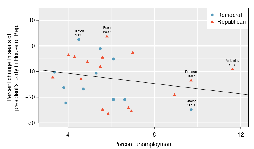
To assess the validity of this claim, we can compile historical data and look for a connection. We consider every midterm election from 1898 to 2010, with the exception of those elections during the Great Depression. Figure \(\PageIndex{1}\) shows these data and the least-squares regression line:
\[\text {% change in House seats for President's party}\]
\[= -6.71 - 1.00 \times \text {(unemployment rate)}\]
We consider the percent change in the number of seats of the President's party (e.g. percent change in the number of seats for Democrats in 2010) against the unemployment rate.

Examining the data, there are no clear deviations from linearity, the constant variance condition, or in the normality of residuals (though we don't examine a normal probability plot here). While the data are collected sequentially, a separate analysis was used to check for any apparent correlation between successive observations; no such correlation was found.
Exercise \(\PageIndex{1}\)
The data for the Great Depression (1934 and 1938) were removed because the unemployment rate was 21% and 18%, respectively. Do you agree that they should be removed for this investigation? Why or why not?
- Answer
-
We will provide two considerations. Each of these points would have very high leverage on any least-squares regression line, and years with such high unemployment may not help us understand what would happen in other years where the unemployment is only modestly high. On the other hand, these are exceptional cases, and we would be discarding important information if we exclude them from a final analysis.
There is a negative slope in the line shown in Figure \(\PageIndex{1}\). However, this slope (and the y-intercept) are only estimates of the parameter values. We might wonder, is this convincing evidence that the "true" linear model has a negative slope? That is, do the data provide strong evidence that the political theory is accurate? We can frame this investigation into a one-sided statistical hypothesis test:
- H0: \(\beta _1 = 0\). The true linear model has slope zero.
- HA: \(\beta _1 < 0\). The true linear model has a slope less than zero. The higher the unemployment, the greater the losses for the President's party in the House of Representatives.
We would reject H0 in favor of HA if the data provide strong evidence that the true slope parameter is less than zero. To assess the hypotheses, we identify a standard error for the estimate, compute an appropriate test statistic, and identify the p-value.
Understanding regression output from software
Just like other point estimates we have seen before, we can compute a standard error and test statistic for \(\beta_1\). We will generally label the test statistic using a T, since it follows the t distribution.
We will rely on statistical software to compute the standard error and leave the explanation of how this standard error is determined to a second or third statistics course. Table \(\PageIndex{1}\) shows software output for the least squares regression line in Figure \(\PageIndex{1}\). The row labeled unemp represents the information for the slope, which is the coefficient of the unemployment variable.
| Estimate | Std. Error | t value | Pr(>|t|) | |
|---|---|---|---|---|
| (Intercept) | -6.7142 |
5.4567 |
-1.23 |
0.2300 |
| unemp | -1.0010 | 0.8717 | -1.15 | 0.2617 |
Example \(\PageIndex{2}\)
What do the first and second columns of Table \(\PageIndex{1}\) represent?
Solution
The entries in the first column represent the least squares estimates, \(\beta_0\) and \(\beta_1\), and the values in the second column correspond to the standard errors of each estimate.
We previously used a t test statistic for hypothesis testing in the context of numerical data. Regression is very similar. In the hypotheses we consider, the null value for the slope is 0, so we can compute the test statistic using the T (or Z) score formula:
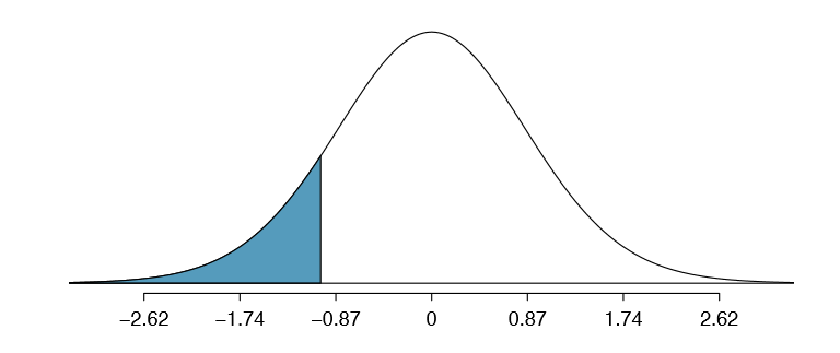
\[T = \frac {\text {estimate - null value}}{SE} = \frac {-1.0010 - 0}{0.8717} = -1.15 \nonumber\]
We can look for the one-sided p-value - shown in Figure \(\PageIndex{2}\) - using the probability table for the t distribution in Appendix B.2

Exercise \(\PageIndex{2}\)
Table \(\PageIndex{1}\) offers the degrees of freedom for the test statistic T: df = 25. Identify the p-value for the hypothesis test.
- Answer
-
Add answer text here and it will automatically be hidden if you have a "AutoNum" template active on the page.
Looking in the 25 degrees of freedom row in Appendix B.2, we see that the absolute value of the test statistic is smaller than any value listed, which means the tail area and therefore also the p-value is larger than 0.100 (one tail!). Because the p-value is so large, we fail to reject the null hypothesis. That is, the data do not provide convincing evidence that a higher unemployment rate has any correspondence with smaller or larger losses for the President's party in the House of Representatives in midterm elections.
We could have identified the t test statistic from the software output in Table \(\PageIndex{1}\), shown in the second row (unemp) and third column (t value). The entry in the second row and last column in Table \(\PageIndex{1}\) represents the p-value for the two-sided hypothesis test where the null value is zero. The corresponding one-sided test would have a p-value half of the listed value.
Inference for regression
We usually rely on statistical software to identify point estimates and standard errors for parameters of a regression line. After verifying conditions hold for fitting a line, we can use the methods learned in Section 5.3 for the t distribution to create con dence intervals for regression parameters or to evaluate hypothesis tests.
Caution: Don't carelessly use the p-value from regression output
The last column in regression output often lists p-values for one particular hypothesis: a two-sided test where the null value is zero. If your test is one-sided and the point estimate is in the direction of HA, then you can halve the software's p-value to get the one-tail area. If neither of these scenarios match your hypothesis test, be cautious about using the software output to obtain the p-value.
Example \(\PageIndex{3}\)
Examine Figure 7.16, which relates the Elmhurst College aid and student family income. How sure are you that the slope is statistically significantly different from zero? That is, do you think a formal hypothesis test would reject the claim that the true slope of the line should be zero?
Solution
While the relationship between the variables is not perfect, there is an evident decreasing trend in the data. This suggests the hypothesis test will reject the null claim that the slope is zero.
Exercise \(\PageIndex{3}\)
Table \(\PageIndex{2}\) shows statistical software output from tting the least squares regression line shown in Figure 7.16. Use this output to formally evaluate the following hypotheses.
- H0: The true coefficient for family income is zero.
- HA: The true coefficient for family income is not zero.
| Estimate | Std. Error | t value |
Pr(>|t|) |
|
|---|---|---|---|---|
|
(Intercept) family_income |
24.3193 -0.0431 |
1.2915 0.0108 |
18.83 -3.98 |
0.0000 0.0002 |
- Answer
-
We look in the second row corresponding to the family income variable. We see the point estimate of the slope of the line is -0.0431, the standard error of this estimate is 0.0108, and the t test statistic is -3.98. The p-value corresponds exactly to the two-sided test we are interested in: 0.0002. The p-value is so small that we reject the null hypothesis and conclude that family income and nancial aid at Elmhurst College for freshman entering in the year 2011 are negatively correlated and the true slope parameter is indeed less than 0, just as we believed in Example 7.27.
TIP: Always check assumptions
If conditions for tting the regression line do not hold, then the methods presented here should not be applied. The standard error or distribution assumption of the point estimate - assumed to be normal when applying the t test statistic - may not be valid.
An alternative Test Statistic
We considered the t test statistic as a way to evaluate the strength of evidence for a hypothesis test in Section 7.4.2. However, we could focus on R2. Recall that R2 described the proportion of variability in the response variable (y) explained by the explanatory variable (x). If this proportion is large, then this suggests a linear relationship exists between the variables. If this proportion is small, then the evidence provided by the data may not be convincing.
This concept - considering the amount of variability in the response variable explained by the explanatory variable - is a key component in some statistical techniques. The analysis of variance (ANOVA) technique introduced in Section 5.5 uses this general principle. The method states that if enough variability is explained away by the categories, then we would conclude the mean varied between the categories. On the other hand, we might not be convinced if only a little variability is explained. ANOVA can be further employed in advanced regression modeling to evaluate the inclusion of explanatory variables, though we leave these details to a later course.


