12.5: Chapter 12 Exercises

Chapter 12 Exercises

1. The correlation coefficient, \(r\), is a number between _______________.

a) -1 and 1
b) -10 and 10
c) 0 and 10
d) 0 and \(\infty\)
e) 0 and 1
f) \(-\infty\) and \(\infty\)

2. To test the significance of the correlation coefficient, we use the t-distribution with how many degrees of freedom?

a) \(n - 1\)
b) \(n\)
c) \(n + 1\)
d) \(n - 2\)
e) \(n_{1} + n_{2} - 2\)

3. What are the hypotheses for testing to see if a correlation is statistically significant?

a) \(H_{0}: r = 0 \quad \ \ \ H_{1}: r \neq 0\)
b) \(H_{0}: \rho = 0 \quad \ \ \ H_{1}: \rho \neq 0\)
c) \(H_{0}: \rho = \pm 1 \quad H_{1}: \rho \neq \pm 1\)
d) \(H_{0}: r = \pm 1 \quad H_{1}: r \neq \pm 1\)
e) \(H_{0}: \rho = 0 \quad \ \ \ H_{1}: \rho = 1\)

4. The coefficient of determination is a number between _______________.

a) -1 and 1
b) -10 and 10
c) 0 and 10
d) 0 and \(\infty\)
e) 0 and 1
f) \(-\infty\) and \(\infty\)

5. Which of the following is not a valid linear regression equation?

a) \(\hat{y} = -5 + \frac{2}{9} x\)
b) \(\hat{y} = 3x + 2\)
c) \(\hat{y} = \frac{2}{9} - 5x\)
d) \(\hat{y} = 5 + 0.4 x\)

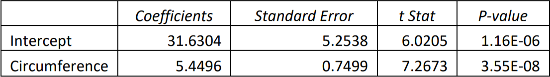
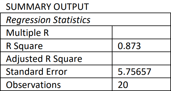
6. Body frame size is determined by a person's wrist circumference in relation to height. A researcher measures the wrist circumference and height of a random sample of individuals. The data is displayed below. Use \(\alpha\) = 0.05.

a) What is the value of the test statistic to see if the correlation is statistically significant?

i. 6.0205
ii. 1.16E-06
iii. 3.55E-08
iv. 5.2538
v. 7.2673
vi. 0.7499
vii. 0.7938

b) What is the correct p-value and conclusion for testing if there is a significant correlation?

i. 1.16E-06; there is a significant correlation.
ii. 3.55E-08; there is a significant correlation.
iii. 1.16E-06; There is not a significant correlation.
iv. 3.55E-08, There is not a significant correlation.
v. 0.7938, There is a significant correlation.
vi. 0.7938, There is not a significant correlation.

7. Bone mineral density and cola consumption have been recorded for a sample of patients. Let \(x\) represent the number of colas consumed per week and \(y\) the bone mineral density in grams per cubic centimeter. Assume the data is normally distributed. Calculate the correlation coefficient.

\(x\)	1	2	3	4	5	6	7	8	9	10	11
\(y\)	0.883	0.8734	0.8898	0.8852	0.8816	0.863	0.8634	0.8648	0.8552	0.8546	0.862

8. A teacher believes that the third homework assignment is a key predictor of how well students will do on the midterm. Let \(x\) represent the third homework score and y the midterm exam score. A random sample of last term’s students were selected and their grades are shown below. Assume scores are normally distributed. Use \(\alpha\) = 0.05.

HW3	Midterm		HW3	Midterm		HW3	Midterm
13.1	59		6.4	43		20	86
21.9	87		20.2	79		15.4	73
8.8	53		21.8	84		25	93
24.3	95		23.1	92		9.7	52
5.4	39		22	87		15.1	70
13.2	66		11.4	54		15	65
20.9	89		14.9	71		16.8	77
18.5	78		18.4	76		20.1	78

a) State the hypotheses to test for a significant correlation.
b) Compute the correlation coefficient.
c) Compute the p-value to see if there is a significant correlation.
d) State the correct decision.
e) Is there a significant correlation?
f) Compute the coefficient of determination.
g) Write a sentence interpreting \(R^{2}\).
h) Does doing poorly on homework 3 cause a student to do poorly on the midterm exam? Explain.
i) Find the standard error of estimate.

9. The sum of the residuals should be ________.

a) a
b) b
c) 0
d) 1
e) \(r\)

10. An object is thrown from the top of a building. The following data measure the height of the object from the ground for a five-second period. Calculate the correlation coefficient.

Seconds	0.5	1	1.5	2	2.5	3	3.5	4	4.5	5
Height	112.5	110.875	106.8	100.275	91.3	79.875	70.083	59.83	30.65	0

11. A teacher believes that the third homework assignment is a key predictor of how well students will do on the midterm. Let \(x\) represent the third homework score and \(y\) the midterm exam score. A random sample of last term’s students were selected and their grades are shown below. Assume scores are normally distributed. Use \(\alpha\) = 0.05.

HW3	Midterm		HW3	Midterm		HW3	Midterm
13.1	59		6.4	43		20	86
21.9	87		20.2	79		15.4	73
8.8	53		21.8	84		25	93
24.3	95		23.1	92		9.7	52
5.4	39		22	87		15.1	70
13.2	66		11.4	54		15	65
20.9	89		14.9	71		16.8	77
18.5	78		18.4	76		20.1	78

a) Compute the regression equation.
b) Compute the predicted midterm score when the homework 3 score is 15.
c) Compute the residual for the point \((15, 65)\).
d) Find the 95% prediction interval for the midterm score when the homework 3 score is 15.

12. Body frame size is determined by a person's wrist circumference in relation to height. A researcher measures the wrist circumference and height of a random sample of individuals. The data is displayed below.

a) Which is the correct regression equation?

i. \(\hat{y} = 31.6304 + 5.4496\)
ii. \(\hat{y} = 31.6304 + 5.4496 x\)
iii. \(\hat{y} = 5.4496 + 31.6304 x\)
iv. \(\hat{y} = 31.6304 + 5.2538 x\)
v. \(y = 31.6304 + 5.4496 x\)

b) What is the predicted height (in inches) for a person with a wrist circumference of 7 inches?
c) Which number is the standard error of estimate?
d) Which number is the coefficient of determination?
e) Compute the correlation coefficient.
f) What is the correct test statistic for testing if the slope is significant \(H_{1}: \beta_{1} \neq 0\)?
g) What is the correct p-value for testing if the slope is significant \(H_{1}: \beta_{1} \neq 0\)?
h) At the 5% level of significance, is there a significant relationship between wrist circumference and height?

13. Bone mineral density and cola consumption have been recorded for a sample of patients. Let \(x\) represent the number of colas consumed per week and \(y\) the bone mineral density in grams per cubic centimeter. Assume the data is normally distributed. Calculate the coefficient of determination.

\(x\)	1	2	3	4	5	6	7	8	9	10	11
\(y\)	0.883	0.8734	0.8898	0.8852	0.8816	0.863	0.8634	0.8648	0.8552	0.8546	0.862

14. Bone mineral density and cola consumption have been recorded for a sample of patients. Let \(x\) represent the number of colas consumed per week and \(y\) the bone mineral density in grams per cubic centimeter. Assume the data is normally distributed. A regression equation for the following data is \(\hat{y} = 0.8893 - 0.0031x\). Which is the best interpretation of the slope coefficient?

\(x\)	1	2	3	4	5	6	7	8	9	10	11
\(y\)	0.883	0.8734	0.8898	0.8852	0.8816	0.863	0.8634	0.8648	0.8552	0.8546	0.862

a) For every additional average weekly soda consumption, a person’s bone density increases by 0.0031 grams per cubic centimeter.
b) For every additional average weekly soda consumption, a person’s bone density decreases by 0.0031 grams per cubic centimeter.
c) For an increase of 0.8893 in the average weekly soda consumption, a person’s bone density decreases by 0.0031 grams per cubic centimeter.
d) For every additional average weekly soda consumption, a person’s bone density decreases by 0.8893 grams per cubic centimeter.

15. Which residual plot has the best linear regression model?

a) a
b) b
c) c
d) d
e) e
f) f

16. An object is thrown from the top of a building. The following data measure the height of the object from the ground for a five-second period.

Seconds	0.5	1	1.5	2	2.5	3	3.5	4	4.5	5
Height	112.5	110.875	106.8	100.275	91.3	79.875	70.083	59.83	30.65	0

The following four plots were part of the regression analysis.

There is a statistically significant correlation between time and height, \(r = -0.942\), p-value = 0.0000454. Should linear regression be used for this data? Why or why not? Choose the correct answer.

a) Yes, the p-value indicates that there is a significant correlation so we can use linear regression.
b) Yes, the normal probability plot has a nice curve to it.
c) Yes, there is a nice straight line in the line fit plot.
d) No, there is a curve in the residual plot, normal plot and the scatterplot.

17. The following data represent the leaching rates (percent of lead extracted vs. time in minutes) for lead in solutions of magnesium chloride \((\mathrm{MgCl}_{2})\). Use \(\alpha = 0.05\).

Time \((x)\)	4	8	16	30	60	120
Percent Extracted \((y)\)	1.2	1.6	2.3	2.8	3.6	4.4

a) State the hypotheses to test for a significant correlation.
b) Compute the correlation coefficient.
c) Compute the p-value to see if there is a significant correlation.
d) State the correct decision.
e) Is there a significant correlation?
f) Compute the coefficient of determination.
g) Compute the regression equation.
h) Compute the 95% prediction interval for 100 minutes.
i) Write a sentence interpreting this interval using units and context.

18. Bone mineral density and cola consumption have been recorded for a sample of patients. Let x represent the number of colas consumed per week and y the bone mineral density in grams per cubic centimeter. Assume the data is normally distributed. What is the residual for the observed point \((7, 0.8634)\).

\(x\)	1	2	3	4	5	6	7	8	9	10	11
\(y\)	0.883	0.8734	0.8898	0.8852	0.8816	0.863	0.8634	0.8648	0.8552	0.8546	0.862

19. A study was conducted to determine if there was a linear relationship between a person's age and their peak heart rate. Use \(\alpha = 0.05\).

Age \((x)\)	16	26	32	37	42	53	48	21
Peak Heart Rate \((y)\)	220	194	193	178	172	160	174	214

a) What is the estimated regression equation that relates number of hours worked and test scores for high school students.
b) Interpret the slope coefficient for this problem.
c) Compute and interpret the coefficient of determination.
d) Compute the coefficient of nondetermination.
e) Compute the standard error of estimate.
f) Compute the correlation coefficient.
g) Compute the 95% Prediction Interval for peak heart rate for someone who is 25 years old.

20. The following data represent the weight of a person riding a bike and the rolling distance achieved after going down a hill without pedaling.

Weight (lbs)	59	84	97	56	103	87	88	92	53	66	71	100
Rolling distance (m)	26	43	48	20	59	44	48	46	28	32	39	49

a) Can it be concluded at a 0.05 level of significance that there is a linear correlation between the two variables?
b) Using the regression line for this problem, find the predicted bike rolling distance for a person that weighs 110 lbs.
c) Find the 99% prediction interval for bike rolling distance for a person that weighs 110 lbs.

21. Body frame size is determined by a person's wrist circumference in relation to height. A researcher measures the wrist circumference and height of a random sample of individuals. The Excel output and scatterplot are displayed below. Find the regression equation and predict the height (in inches) for a person with a wrist circumference of 7 inches. Then, compute the residual for the point \((7, 75)\).

22. It has long been thought that the length of one’s femur is positively correlated to the length of one’s tibia. The following are data for a classroom of students who measured each (approximately) in inches. A significant linear correlation was found between the two variables. Find the 90% prediction interval for the length of someone’s tibia when it is known that their femur is 23 inches long.

Femur Length	18.7	20.5	16.2	15.0	19.0	21.3	21.0	14.3	15.8	18.8	18.7
Tibia Length	14.2	15.9	13.1	12.4	16.2	15.8	16.2	12.1	13.0	14.3	13.8

23. The data below represent the driving speed (mph) of a vehicle and the corresponding gas mileage (mpg) for several recorded instances.

Driving Speed	Gas Mileage		Driving Speed	Gas Mileage
57	21.8		62	21.5
66	20.9		66	20.5
42	25.0		67	23.0
34	26.2		52	19.4
44	24.3		49	25.3
44	26.3		48	24.3
25	26.1		41	28.4
20	27.2		38	29.6
24	23.5		26	32.5
42	22.6		24	30.8
52	19.4		21	28.8
54	23.9		19	33.5
60	24.8		24	25.1

a) Do a hypothesis test to see if there is a significant correlation. Use \(\alpha = 0.10\).
b) Compute the standard error of estimate.
c) Compute the regression equation and use it to find the predicted gas mileage when a vehicle is driving at 77 mph.
d) Compute the 90% prediction interval for gas mileage when a vehicle is driving at 77 mph.

24. The following data represent the age of a car and the average monthly cost for repairs. A significant linear correlation is found between the two variables. Use the data to find a 95% prediction interval for the monthly cost of repairs for a vehicle that is 15 years old.

Age of Car (yrs)	1	2	3	4	5	6	7	8	9	10
Monthly Cost ($)	25	34	42	45	55	71	82	88	87	90

25. In a sample of 20 football players for a college team, their weight and 40-yard-dash time in minutes were recorded.

Weight (lbs)	40-Yard Dash (min)		Weight (lbs)	40-Yard Dash (min)
285	5.95		195	4.85
185	4.99		254	5.12
165	4.92		140	4.87
188	4.77		212	5.05
160	4.52		158	4.75
156	4.67		188	4.87
256	5.22		134	4.53
169	4.95		205	4.92
210	5.06		178	4.88
165	4.83		159	4.79

a) Do a hypothesis test to see if there is a significant correlation. Use \(\alpha = 0.01\).
b) Compute the standard error of estimate.
c) Compute the regression equation and use it to find the predicted 40-yard-dash time for a football player that is 200 lbs.
d) Compute the 99% prediction interval for a football player that is 200 lbs.
e) Write a sentence interpreting the prediction interval.

26. The following data represent the enrollment at a small college during its first ten years of existence. A significant linear relationship is found between the two variables. Find a 90% prediction interval for the enrollment after the college has been open for 14 years.

Years	1	2	3	4	5	6	7	8	9	10
Enrollment	856	842	923	956	940	981	1025	996	1057	1088

27. A new fad diet called Trim-to-the-MAX is running some tests that they can use in advertisements. They sample 25 of their users and record the number of days each has been on the diet along with how much weight they have lost in pounds. The data is below. A significant linear correlation was found between the two variables. Find the 95% prediction interval for the weight lost when a person has been on the diet for 60 days.

Days on Diet	7	12	16	19	25	34	39	43	44	49
Weight Loss	5	7	12	15	20	25	24	29	33	35

28. An elementary school uses the same system to test math skills at their school throughout the course of the 5 grades at their school. The age and score (out of 100) of several students is displayed below. A significant linear relationship is found between the student’s age and their math score. Find a 90% prediction interval for the score a student would earn given that they are 5 years old.

Student Age	6	6	7	8	8	9	10	11	11
Math Score	54	42	50	61	67	65	71	72	79

29. The intensity (in candelas) of a 100-watt light bulb was measured by a sensing device at various distances (in meters) from the light source. A linear regression was run and the following residual plot was found.

a) Is linear regression a good model to use?
b) Write a sentence explaining your answer.

30. The table below shows the percentage of adults in the United States who were married before age 24 for the years shown. A significant linear relationship was found between the two variables.

Year	1960	1965	1970	1975	1980	1985	1990	1995	2000	2005
% Married Before 24 Years Old	52.1	51.3	45.9	46.3	40.8	38.1	34.0	32.6	28.1	25.5

a) Compute the regression equation.
b) Predict the percentage of adults who married before age 24 in the United States in 2015.
c) Compute the 95% prediction interval for the percentage of adults who married before age 24 in the United States in 2015.

31. A nutritionist feels that what mothers eat during the months they are nursing their babies is important for healthy weight gain of their babies. She samples several of her clients and records their average daily caloric intake for the first three months of their babies’ lives and also records the amount of weight the babies gained in those three months. The data are below.

Daily Calories	1523	1649	1677	1780	1852	2065	2096	2145	2378
Baby's Weight Gain (lbs)	4.62	4.77	4.62	5.12	5.81	5.34	5.89	5.96	6.05

a) Compute the regression equation.
b) Test to see if the slope is significantly different from zero, using \(\alpha = 0.05\).
c) Predict the weight gain of a baby whose mother gets 2,500 calories per day.
d) Compute the 95% prediction interval for the weight gain of a baby whose mother gets 2,500 calories per day.

32. The data below show the predicted average high temperature \(({}^{\circ} \mathrm{F})\) per month by the Farmer’s Almanac in Portland, Oregon alongside the actual high temperature per month that occurred.

Farmer's Almanac	45	50	57	62	69	72	81	90	78	64	51	48
Actual High	46	52	60	61	72	78	82	95	85	68	52	49

a) Compute the regression equation.
b) Test to see if the slope is significantly different from zero, using \(\alpha = 0.01\).
c) Predict the high temperature in the coming year, given that the Farmer’s Almanac is predicting the high to be \(58^{\circ} \mathrm{F}\).
d) Compute the 99% prediction interval for the actual high temperature in the coming year, given that the Farmer’s Almanac is predicting the high to be \(58^{\circ} \mathrm{F}\).

33. In a multiple linear regression problem, p represents:

a) The number of dependent variables in the problem.
b) The probability of success.
c) The number of independent variables in the problem.
d) The probability of failure.
e) The population proportion.

34. The manager of a warehouse found a significant relationship exists between the number of weekly hours clocked \((x_{1}\)), the age of the employee \((x_{2})\), and the productivity of the employee \((y)\) (measured in weekly orders assembled). A multiple regression was run and the following line of best fit was found: \(\hat{y} = 66.238 + 2.7048 x_{1} - 0.7275 x_{2}\). Approximate the productivity level of an employee who clocked 61 hours in a given week and is 59 years old.

35. A multiple regression test concludes that there is a linear relationship and finds the following line of best fit: \(\hat{y} = -53.247 + 12.594 x_{1} - 0.648 x_{2} + 4.677 x_{3}\). Use the line of best fit to approximate \(y\) when \(x_{1} = 5\), \(x_{2} = 12\), \(x_{3} = 2\).

36. A career counselor feels that the strongest predictors of a student’s success after college are class attendance \((x_{1})\) (recorded as a percent) and GPA \((x_{2})\). To test this, she samples clients after they have found a job and lets the dependent variable be the number of weeks it took them to find a job. A multiple regression was run and the following line of best fit was found \(\hat{y} = 38.6609 - 0.3345 x_{1} - 1.0743 x_{2}\). Predict the number of weeks it will take a client to find a job, given that she had a 94% \((x_{1} = 94)\) attendance rate in college and a 3.82 GPA.

37. A study conducted by the American Heart Association provided data on how age, blood pressure and smoking relate to the risk of strokes. The following data is the SPSS output with Age in years \((x_{1})\), Blood Pressure in mmHg \((x_{2})\), Smoker (0 = Nonsmoker, 1 = Smoker) \((x_{3})\) and the Risk of a Stroke as a percent \((y)\).

a) Use \(\alpha = 0.05\) to test the claim that the regression model is significant. State the hypotheses, test statistic, p-value, decision and summary.
b) Use the estimated regression equation to predict the stroke risk for a 70-year-old smoker with a blood pressure of 180.
c) Interpret the slope coefficient for age.
d) Find the adjusted coefficient of determination.

38. Use technology to run a multiple linear regression with a dependent variable of annual salary for adults with full-time jobs in San Francisco and independent variables of years of education completed and age. The data for the sample used is below.

Annual Salary	Years of Education	Age
82,640	17	34
95,854	18	42
152,320	21	39
49,165	13	25
31,120	12	31
67,500	16	32
42,590	12	28
57,245	14	55
58,940	16	45
67,250	18	40
56,120	16	39
38,955	12	34
74,650	16	33
53,495	16	29
67,210	16	30
79,365	16	50
96,045	18	51
78,472	14	60
124,975	21	52
43,125	12	36

a) Test to see if the overall model is significant using \(\alpha = 0.05\).
b) Compute the predicted salary for a 35-year-old with 16 years of education.
c) Compute the adjusted coefficient of determination.
d) Are all the independent variables statistically significant? Explain.

39. A study was conducted to determine if there was a linear relationship between a person's weight in pounds with their gender, height and activity level. A person’s gender was recorded as a 0 for anyone who identified as male and 1 for those who did not identify as male. Height was measured in inches. Activity level was coded as 1, 2, or 3; the more active the person was, the higher the value.

a) Interpret the slope coefficient for height.
b) Predict the weight for a male who is 70 inches tall and has an activity level of 2.
c) Calculate the adjusted coefficient of determination.

40. A professor claims that the number of hours a student studies for their final paired with the number of homework assignments completed throughout the semester (out of 20 total assignment opportunities) is a good predictor of a student’s final exam grade. She collects a sample of students and records the following data.

Final Exam Score	# Hours Studied	HW Completed
85	5.2	19
74	5.1	18
79	4.9	16
62	3.7	12
96	9	17
52	1	12
73	2	15
81	2	16
90	7.25	18
79	4.5	14
83	3	20
76	3.2	17
92	6.8	20
84	6.2	18
50	4.1	10

a) Test the professor’s claim using \(\alpha = 0.05\).
b) Compute the multiple correlation coefficient.
c) Interpret the slope coefficient for number of hours studied.
d) Compute the adjusted coefficient of determination.

Solutions to Odd-Numbered Exercises

1. a

3. b

5. d

7. \(r = 0.8241\)

9. c

11. a) \(\hat{y} = 25.6472 + 2.8212 x\)
b) \(67.9657\)
c) \(-2.9657\)
d) \(61.3248 < y < 74.6065\)

13. \(R^{2} = 0.679\)

15. a

17. a) \(H_{0}: \rho = 0; H_{1}: \rho \neq 0\)
b) \(r = 0.9403\)
c) \(0.0052\)
d) Reject \(H_{0}\)
e) Yes
f) \(R^{2} = 0.8842\)
g) \(\hat{y} = 1.6307 - 0.0257x\)
h) \(2.6154 < y < 5.7852\)
i) We can be 95% confident that the predicted percent of lead extracted in solutions of magnesium chloride at 100 minutes is anywhere between 2.6154 and 5.7852.

19. a) \(\hat{y} = 241.8127 - 1.5618x\)
b) Every year a person ages, their peak heart rate decreases by an average of 1.5618.
c) \(R^{2} = 0.93722\)
d) \(0.06278\)
e) \(5.6924\)
f) \(r = -0.9681\)

21. 5.2224

23. a) \(H_{0}: \rho = 0; H_{1}: \rho \neq 0; t = -5.2514;\) p-value = \(0.000022\).
Reject \(H_{0}\). There is a significant correlation between driving speed of a vehicle and the corresponding gas mileage.
b) 2.49433
c) \(\hat{y} = 32.40313 - 0.1662x\)
d) \(14.8697 < y < 24.3424\)

25. a) \(H_{0}: \rho = 0; H_{1}: \rho \neq 0; t = 6.9083;\) p-value = \(0.000007\).
Reject \(H_{0}\). There is a significant correlation between a football player’s weight and 40-yard-dash time.
b) \(s = 0.160595\)
c) \(\hat{y} = 3.722331 - 0.006396x; 5.0016\)
d) \(4.527 < y < 5.476\)
e) We can be 99% confident that the predicted time for all 200-pound football player’s running time for the 40-yard-dash is between 4.527 and 5.476 minutes.

27. \(36.605 < y < 47.740\)

29. a) No
b) The p-value = 0.00000304 suggests that there is a significant linear relationship between intensity (in candelas) of a 100-watt light bulb was measured by a sensing device at various distances (in meters) from the light source. However, the residual plot clearly shows a nonlinear relationship. Even though we can fit a straight line through the points, we would get a better fit with a curve.

31. a) \(\hat{y} = 1.76267 - 0.001883x\)
b) \(H_{0}: \beta_{1} = 0; H_{1}: \beta_{1} \neq 0; t = 5.0668;\) p-value = \(0.0015\)
Reject \(H_{0}\). There is significant linear relationship between a nursing baby’s weight gain and the calorie intake of the mother.
c) \(6.4693 \mathrm{~lbs}\)
d) \(5.571 < y < 7.368\)

33. c

35. 11.301

37. a) \(H_{0}: \beta_{1} = \beta_{2} = \beta_{3} = 0; H_{1}:\) At least one slope is not zero\(; F = 36.823;\) p-value = \(0.000000204\)
Reject \(H_{0}\). There is a significant relationship between a person’s age, blood pressure and smoking status and the risk of a stroke.
b) \(37.731%\)
c) For each year a person ages, their chance of a stroke increases by 1.077%.
d) \(84.9%\)

39. a) For each additional inch in height, the predicted weight would increase 3.7 pounds.
b) \(171.34 \mathrm{~lbs}\)
c) \(65.56%\)