12.2.6: Conclusion - Simple Linear Regression

A lurking variable is a variable other than the independent or dependent variables that may influence the regression line. For instance, the highly correlated ice cream sales and home burglary rates probably have to do with the season. Hence, linear regression does not imply cause and effect.

Two variables are confounded when their effects on the dependent variable cannot be distinguished from each other. For instance, if we are looking at diet predicting weight, a confounding variable would be age. As a person gets older, they can gain more weight with fewer calories compared to when they were younger. Another example would be predicting someone’s midterm score from hours studied for the exam. Some confounding variables would be GPA, IQ score, and teacher’s difficultly level.

Assumptions for Linear Regression

There are assumptions that need to be met when running simple linear regression. If these assumptions are not met, then one should use more advanced regression techniques.

The assumptions for simple linear regression are:

• The data need to follow a linear pattern.
• The observations of the dependent variable y are independent of one another.
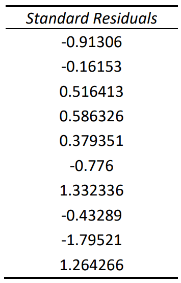
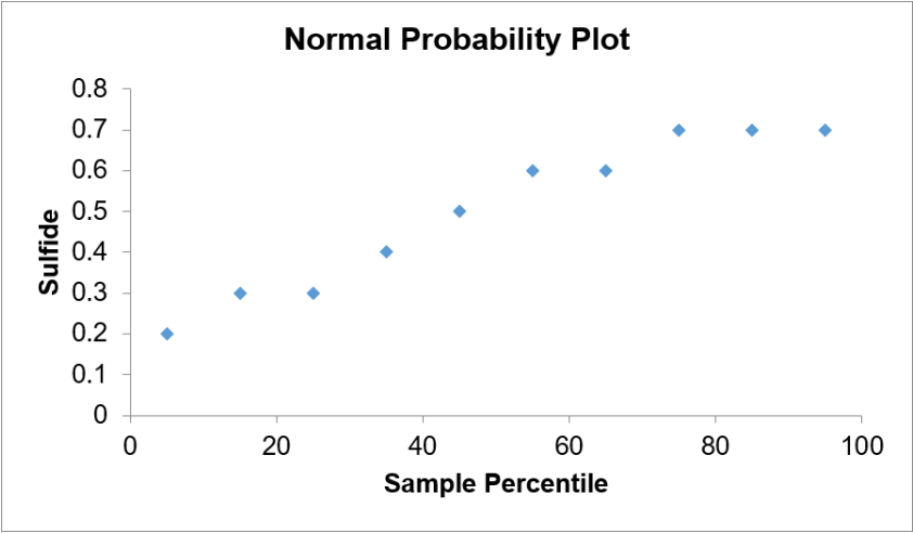
• Residuals are approximately normally distributed.
• The variance of the residuals is constant.

Most software packages will plot the residuals for each \(x\) on the \(y\)-axis against either the \(x\)-variable or \(\hat{y}\) along the \(x\)-axis. This plot is called a residual plot. Residual plots help determine some of these assumptions.

Use technology to compute the residuals and make a residual plot for the hours studied and exam grade data.

Hours Studied for Exam 20 16 20 18 17 16 15 17 15 16 15 17 16 17 14 Grade on Exam 89 72 93 84 81 75 70 82 69 83 80 83 81 84 76

Solution

Plot the residuals.

TI-84: Find the least-squares regression line as described in the previous section. Press [Y=] and clear any equations that are in the \(y\)-editor. Press [2nd] then [STAT PLOT] then press 1 or hit [ENTER] to select Plot1. Select On and press [ENTER] to activate plot 1. For “Type” select the first graph that looks like a scatterplot and press [ENTER]. For “Xlist” enter whichever list where your explanatory variable data is stored. For our example, enter L₁. For “Ylist” press [2nd] [LIST] then scroll down to RESID and press [ENTER]. The calculator automatically computes the residuals and stores them in a list called RESID. Press [ZOOM] then press 9 or scroll down to ZoomStat and press [ENTER].

TI-89: Find the least-squares regression line as described in the previous section. Press [♦] then [F1] (Y=) and clear any equations that are in the \(y\)-editor. In the Stats/List Editor select F2 for the Plots menu. Use cursor keys to highlight 1:Plot Setup. Make sure that the other graphs are turned off by pressing F4 button to remove the check marks. Under “Plot 2” press F1 for the Define menu. In the “Plot Type” menu select “Scatter.” In the “x” space type in the name of your list with the x variable without space, for our example “list1.” In the “y” space press [2ND] [-] for the VAR-LINK menu. Scroll down the list and find “resid” in the “STATVARS” menu. Press [ENTER] twice and you will be returned to the Plot Setup menu. Press F5 ZoomData to display the graph. Press F3 Trace and use the arrow keys to scroll along the different points.

Excel: Run the regression the same as in the last section when testing to see if there is a significant correlation. Type the data into two columns in Excel. Select the Data tab, then Data Analysis, then choose Regression and select OK.

Be careful here, the second column is the \(y\) range, and the first column is the \(x\) range.

Only check the Labels box if you highlight the labels in the input range. The output range is one cell reference where you want the output to start. Check the residuals, residual plots and normal probability plots, then select OK.

Figure 12-21 shows the Excel Output.

Figure 12-21: Output for running a regression in Excel.

Additional output from Excel gives the residuals, residual plot, and normal probability plot; see below.

With this additional output, you can check the assumptions about the residuals. The residual plot is random and the normal probability plot forms an approximately straight line.

Putting It All Together

High levels of hydrogen sulfide \((\mathrm{H}_{2} \mathrm{S})\) in the ocean can be harmful to animal life. It is expensive to run tests to detect these levels. A scientist would like to see if there is a relationship between sulfate \((\mathrm{SO}_{4})\) and \(\mathrm{H}_{2} \mathrm{S}\) levels, since \(\mathrm{SO}_{4}\) is much easier and less expensive to test in ocean water. A sample of \(\mathrm{SO}_{4}\) and \(\mathrm{H}_{2} \mathrm{S}\) were recorded together at different depths in the ocean. The sample is reported below in millimolar (mM). If there were a significant relationship, the scientist would like to predict the \(\mathrm{H}_{2} \mathrm{S}\) level when the ocean has an \(\mathrm{SO}_{4}\) level of 25 mM. Run a complete regression analysis and check the assumptions. If the model is significant, then find the 95% prediction interval to predict the sulfide level in the ocean when the sulfate level is 25 mM.

Sulfate 22.5 27.5 24.6 27.3 23.1 24 24.5 28.4 25.1 24.4 Sulfide 0.6 0.3 0.6 0.4 0.7 0.5 0.7 0.2 0.3 0.7

Solution

Start with a scatterplot to see if a linear relation exists.

Figure 12-22: Scatterplot of sulfide and sulfate level data.

The scatterplot in Figure 12-22 shows a negative linear relationship. Test to see if the linear relationship is statistically significant. Use \(\alpha\) = 0.05. You could use an F- or a t-test. I would recommend the t-test if you are using a TI calculator and an F-test if you are using a computer program like Excel or SPSS. We will do the F-test for the following example.

The hypotheses are:

\(H_{0}: \beta_{1} = 0\)
\(H_{1}: \beta_{1} \neq 0\)

Compute the sum of squares.

\(SS_{xx} = (n-1) s_{x}^{2} = (10 - 1)1.959138^{2} = 34.544\)
\(SS_{yy} = (n-1) s_{y}^{2} = (10 - 1)0.188561^{2} = 0.32\)
\(SS_{xy} = \sum (xy) - n \cdot \bar{x} \cdot \bar{y} = 123.04 - 10 \cdot 25.14 \cdot \cdot 0.5 = -2.66\)

Next, compute the test statistic.

\(\begin{array}{l} & SSR = \frac{\left(SS_{xy}\right)^{2}}{SS_{xx}} = \frac{-2.66^{2}}{34.544} = 0.2048286 \quad\quad\quad\quad & SST = SS_{yy} = 0.32 \\ & SSE = SST - SSR = 0.32 - 0.2048286 = 0.1151714 \\ & df_{T} = n - 1 = 9 & df_{E} = n - p - 1 = 10 - 1 - 1 = 8 \\ & MSR = \frac{SSR}{p} = \frac{0.24829}{1} = = 0.204829 & SE = \frac{SSE}{n-p-1} = \frac{0.115171}{8} = 0.014396 \\ & F = \frac{MSR}{MSE} = \frac{0.204829}{0.014396} = 14.228 \end{array} \)

Compute the p-value. This is a right-tailed F-test with \(df = 1, 8\), which gives a p-value of =F.DIST.RT(14.2277,1,8) = 0.00545.

We could also use Excel to generate the p-value.

The p-value = 0.00545 < \(\alpha\) = 0.05; therefore, reject \(H_{0}\). There is a statistically significant linear relationship between hydrogen sulfide and sulfate levels in the ocean.

From the linear regression, check the assumptions and make sure there are no outliers.

The standardized residuals are between \(-2\) and \(2\), and the scatterplot does not indicate any outliers.

The Normal Probability Plot in Figure 12-23 forms an approximately straight line. This indicates that the residuals are approximately normally distributed.

Figure 12-23: Normal probability plot.

The residual plot in Figure 12-24 has no unusual pattern. This indicates that a linear model would work well for this data.

Figure 12-24: Sulfate residual plot.

Now find and use the regression equation to calculate the 95% prediction interval to predict the sulfide level in the ocean when the sulfate level is 25 mM.

Find the regression equation. Calculate the slope: \(b_{1} = \frac{SS_{xy}}{SS_{xx}} = \frac{-2.66}{34.544} = -0.077\).

Then calculate the \(y\)-intercept: \(b_{0} = \bar{y} - b_{1} \cdot \bar{x} = 0.5 - (-0.077) \cdot 25.14 = 2.43586\).

Put the numbers back into the regression equation and write your answer as: \(\hat{y} = 2.4359 + (-0.077)x\) or as \(\hat{y} = 2.4359 - 0.077x\).

We can use technology to get the regression equation. Coefficients are found in the first column in the computer output.

We would expect variation in our predicted value every time a new sample is used. Find the 95% prediction interval to estimate the sulfide level when the sulfate level is 25 mM.

Use the prediction interval equation \(\hat{y} \pm t_{\alpha / 2} \cdot s \sqrt{\left(1 + \frac{1}{n} + \frac{\left(x - \bar{x}\right)^{2}}{SS_{xx}}\right)}\).

Substitute \(x = 25\) into the equation to get \(\hat{y} = 2.43586 - 0.0770032 \cdot 25 = 0.51078\).

To find \(t_{\alpha/2}\) use your calculator's invT with \(df_{E} = n - 2 = 8\) and left-tail area \(\frac{\alpha}{2} = \frac{0.05}{2} = 0.025\), gives \(t_{0.025} = \pm 2.306004\).

The standard error of estimate \(s = \sqrt{MSE} = \sqrt{0.014396} = 0.11998\), which can also be found using technology.

From the earlier descriptive statistics, we have \(n = 10\), \(\bar{x}= 25.14\), \(SS_{xx} = 34.544\). Substitute each of these values into the prediction interval to get the following:

\(0.51078 \pm 2.306004 \cdot 0.119985 \sqrt{\left(1 + \frac{1}{10} + \frac{(25 - 25.14)^{2}}{34.544}\right)}\)

\(0.51078 \pm 0.290265\)

\(0.2205 < y < 0.8010\)

We can be 95% confident that the true sulfide level in the ocean will be between 0.2205 and 0.801 mM when the sulfate level is 25 mM.

Summary

A simple linear regression should only be performed if you observe visually that there is a linear pattern in the scatterplot and that there is a statistically significant correlation between the independent and dependent variables. Use technology to find the numeric values for the \(y\)-intercept = \(a = b_{0}\) and slope = \(b = b_{1}\), then make sure to use the correct notation when substituting your numbers back in the regression equation \(\hat{y} = b_{0} + b_{1} x\). Another measure of how well the line fits the data is called the coefficient of determination \(R^{2}\). When \(R^{2}\) is close to 1 (or 100%), then the line fits the data very closely. The advantage over using \(R^{2}\) over \(r\) is that we can use \(R^{2}\) for nonlinear regression, whereas \(r\) is only for linear regression.

One should always check the assumptions for regression before using the regression equation for prediction. Make sure that the residual plots have a completely random horizontal band around zero. There should be no patterns in the residual plots such as a sideways V that may indicate a non-constant variance. A pattern like a slanted line, a U, or an upside-down U shape would suggest a non-linear model. Check that the residuals are normally distributed; this is not the same as the population being normally distributed. Check to make sure that there are no outliers. Be careful with lurking and confounding variables.