12.2.1: Hypothesis Test for Linear Regression

To test to see if the slope is significant we will be doing a two-tailed test with hypotheses. The population least squares regression line would be \(y = \beta_{0} + \beta_{1} + \varepsilon\) where \(\beta_{0}\) (pronounced “beta-naught”) is the population \(y\)-intercept, \(\beta_{1}\) (pronounced “beta-one”) is the population slope and \(\varepsilon\) is called the error term.

If the slope were horizontal (equal to zero), the regression line would give the same \(y\)-value for every input of \(x\) and would be of no use. If there is a statistically significant linear relationship then the slope needs to be different from zero. We will only do the two-tailed test, but the same rules for hypothesis testing apply for a one-tailed test.

We will only be using the two-tailed test for a population slope.

The hypotheses are:

\(H_{0}: \beta_{1} = 0\)
\(H_{1}: \beta_{1} \neq 0\)

The null hypothesis of a two-tailed test states that there is not a linear relationship between \(x\) and \(y\). The alternative hypothesis of a two-tailed test states that there is a significant linear relationship between \(x\) and \(y\).

Either a t-test or an F-test may be used to see if the slope is significantly different from zero. The population of the variable \(y\) must be normally distributed.

F-Test for Regression

An F-test can be used instead of a t-test. Both tests will yield the same results, so it is a matter of preference and what technology is available. Figure 12-12 is a template for a regression ANOVA table,

Figure 12-12: Regression ANOVA table template.

where \(n\) is the number of pairs in the sample and \(p\) is the number of predictor (independent) variables; for now this is just \(p = 1\). Use the F-distribution with degrees of freedom for regression = \(df_{R} = p\), and degrees of freedom for error = \(df_{E} = n - p - 1\). This F-test is always a right-tailed test since ANOVA is testing the variation in the regression model is larger than the variation in the error.

Use an F-test to see if there is a significant relationship between hours studied and grade on the exam. Use \(\alpha\) = 0.05.

Hours Studied for Exam 20 16 20 18 17 16 15 17 15 16 15 17 16 17 14 Grade on Exam 89 72 93 84 81 75 70 82 69 83 80 83 81 84 76

Solution

The hypotheses are:

\(H_{0}: \beta_{1} = 0\)
\(H_{1}: \beta_{1} \neq 0\)

Compute the sum of squares.

\(SS_{xx} = 41.6\), \(SS_{yy} = 631.7333\), \(SS_{xy} = 133.8\), \(n = 15\) and \(p = 1\)

\(SSR = \frac{\left(SS_{xy}\right)^{2}}{SS_{xx}} = \frac{(133.8)^{2}}{41.6} = 430.3471154\)

\(SSE = SST - SSR = 631.7333 - 430.3471154 = 201.3862\)

\(SST = SS_{yy} = 631.7333\)

Compute the degrees freedom.

\(df_{T} = n - 1 = 14 \quad\quad df_{E} = n - p - 1 = 15 - 1 - 1 = 13\)

Compute the mean squares.

\(MSR = \frac{SSR}{p} = \frac{430.3471154}{1} = 430.3471154 \quad\quad MSE = \frac{SSE}{n-p-1} = \frac{201.3862}{13} = 15.4912\)

Compute the Test Statistic

\(F = \frac{MSR}{MSE} = \frac{430.3471154}{15.4912} = 27.7801\)

Substitute the numbers into the ANOVA table:

This is a right-tailed F-test with \(df = 1, 13\) and \(\alpha\) = 0.05, which gives a critical value of 4.667.

In Excel we can find the critical value by using the function =F.INV.RT(0.05,1,13) = 4.667.

Or use the online calculator at https://homepage.divms.uiowa.edu/~mbognar/applets/f.html to visualize the critical value, as shown in Figure 12-13. It is hard to see the shaded tail in the following picture above the test statistic since the F-distribution is so close to the \(x\)-axis after 3, but it has the right-tail shaded from 4.667 and greater.

Figure 12-13: F-distribution graph generated by online calculator, with the input values displayed.

The test statistic 27.78 is even further out in the tail than the critical value, so we would reject \(H_{0}\). At the 5% level of significance, there is a statistically significant relationship between hours studied and grade on a student’s final exam.

The p-value could also be used to make the decision. The p-value method would use the function =F.DIST.RT(27.78,1,13) = 0.00015 in Excel. The p-value is less than \(\alpha\) = 0.05, which also verifies that we reject \(H_{0}\).

The following is the output from Excel and SPSS. Note the same ANOVA table information is shown but the columns are in a different order.

Excel

SPSS

T-Test for Regression

If the regression equation has a slope of zero, then every \(x\) value will give the same \(y\) value and the regression equation would be useless for prediction. We should perform a t-test to see if the slope is significantly different from zero before using the regression equation for prediction. The numeric value of t will be the same as the t-test for a correlation. The two test statistic formulas are algebraically equal; however, the formulas are different and we use a different parameter in the hypotheses.

The formula for the t-test statistic is \(t = \frac{b_{1}}{\sqrt{ \left(\frac{MSE}{SS_{xx}}\right) }}\)

Use the t-distribution with degrees of freedom equal to \(n - p - 1\).

The t-test for slope has the same hypotheses as the F-test:

\(H_{0}: \beta_{1} = 0\)
\(H_{1}: \beta_{1} \neq 0\)

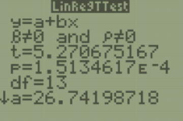
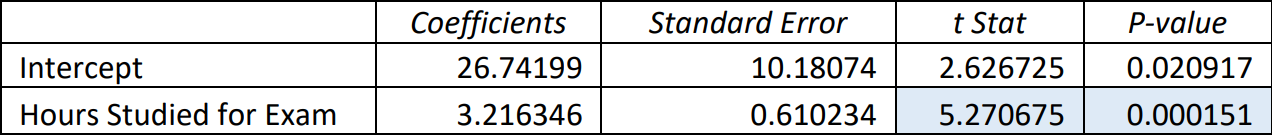
Use a t-test to see if there is a significant relationship between hours studied and grade on the exam, use \(\alpha\) = 0.05.

Hours Studied for Exam 20 16 20 18 17 16 15 17 15 16 15 17 16 17 14 Grade on Exam 89 72 93 84 81 75 70 82 69 83 80 83 81 84 76

Solution

The hypotheses are:

\(H_{0}: \beta_{1} = 0\)
\(H_{1}: \beta_{1} \neq 0\)

Find the critical value using \(df_{E} = n - p - 1 = 13\) for a two-tailed test \(\alpha\) = 0.05 inverse t-distribution to get the critical values \(\pm 2.160\).

Draw the sampling distribution and label the critical values, as shown in Figure 12-14.

Figure 12-14: Graph of t-distribution with labeled critical values.

The critical value is the same as we found using the t-test for correlation.

Next, find the test statistic \(t = \frac{b_{1}}{\sqrt{ \left(\frac{MSE}{SS_{xx}}\right) }} = \frac{3.216346}{\sqrt{ \left(\frac{15.4912}{41.6}\right) }}\) = 5.271\).

The test statistic value is the same value of the t-test for correlation even though they used different formulas. We look in the same place using technology as the correlation test.

The test statistic is greater than the critical value of 2.160 and in the rejection region. The decision is to reject \(H_{0}\).

Summary: At the 5% significance level, there is enough evidence to support the claim that there is a significant linear relationship (correlation) between the number of hours studied for an exam and exam scores. The p-value method could also be used to find the same decision.

The p-value = 0.00015, the same as the previous tests. We will use technology for the p-value method. In the SPSS output, they use Sig. for the p-value.

Excel

SPSS