
11.3: Two-Way ANOVA (Factorial Design)
- Page ID
- 24073

\( \newcommand{\vecs}[1]{\overset { \scriptstyle \rightharpoonup} {\mathbf{#1}} } \)
\( \newcommand{\vecd}[1]{\overset{-\!-\!\rightharpoonup}{\vphantom{a}\smash {#1}}} \)
\( \newcommand{\dsum}{\displaystyle\sum\limits} \)
\( \newcommand{\dint}{\displaystyle\int\limits} \)
\( \newcommand{\dlim}{\displaystyle\lim\limits} \)
\( \newcommand{\id}{\mathrm{id}}\) \( \newcommand{\Span}{\mathrm{span}}\)
( \newcommand{\kernel}{\mathrm{null}\,}\) \( \newcommand{\range}{\mathrm{range}\,}\)
\( \newcommand{\RealPart}{\mathrm{Re}}\) \( \newcommand{\ImaginaryPart}{\mathrm{Im}}\)
\( \newcommand{\Argument}{\mathrm{Arg}}\) \( \newcommand{\norm}[1]{\| #1 \|}\)
\( \newcommand{\inner}[2]{\langle #1, #2 \rangle}\)
\( \newcommand{\Span}{\mathrm{span}}\)
\( \newcommand{\id}{\mathrm{id}}\)
\( \newcommand{\Span}{\mathrm{span}}\)
\( \newcommand{\kernel}{\mathrm{null}\,}\)
\( \newcommand{\range}{\mathrm{range}\,}\)
\( \newcommand{\RealPart}{\mathrm{Re}}\)
\( \newcommand{\ImaginaryPart}{\mathrm{Im}}\)
\( \newcommand{\Argument}{\mathrm{Arg}}\)
\( \newcommand{\norm}[1]{\| #1 \|}\)
\( \newcommand{\inner}[2]{\langle #1, #2 \rangle}\)
\( \newcommand{\Span}{\mathrm{span}}\) \( \newcommand{\AA}{\unicode[.8,0]{x212B}}\)
\( \newcommand{\vectorA}[1]{\vec{#1}} % arrow\)
\( \newcommand{\vectorAt}[1]{\vec{\text{#1}}} % arrow\)
\( \newcommand{\vectorB}[1]{\overset { \scriptstyle \rightharpoonup} {\mathbf{#1}} } \)
\( \newcommand{\vectorC}[1]{\textbf{#1}} \)
\( \newcommand{\vectorD}[1]{\overrightarrow{#1}} \)
\( \newcommand{\vectorDt}[1]{\overrightarrow{\text{#1}}} \)
\( \newcommand{\vectE}[1]{\overset{-\!-\!\rightharpoonup}{\vphantom{a}\smash{\mathbf {#1}}}} \)
\( \newcommand{\vecs}[1]{\overset { \scriptstyle \rightharpoonup} {\mathbf{#1}} } \)
\(\newcommand{\longvect}{\overrightarrow}\)
\( \newcommand{\vecd}[1]{\overset{-\!-\!\rightharpoonup}{\vphantom{a}\smash {#1}}} \)
\(\newcommand{\avec}{\mathbf a}\) \(\newcommand{\bvec}{\mathbf b}\) \(\newcommand{\cvec}{\mathbf c}\) \(\newcommand{\dvec}{\mathbf d}\) \(\newcommand{\dtil}{\widetilde{\mathbf d}}\) \(\newcommand{\evec}{\mathbf e}\) \(\newcommand{\fvec}{\mathbf f}\) \(\newcommand{\nvec}{\mathbf n}\) \(\newcommand{\pvec}{\mathbf p}\) \(\newcommand{\qvec}{\mathbf q}\) \(\newcommand{\svec}{\mathbf s}\) \(\newcommand{\tvec}{\mathbf t}\) \(\newcommand{\uvec}{\mathbf u}\) \(\newcommand{\vvec}{\mathbf v}\) \(\newcommand{\wvec}{\mathbf w}\) \(\newcommand{\xvec}{\mathbf x}\) \(\newcommand{\yvec}{\mathbf y}\) \(\newcommand{\zvec}{\mathbf z}\) \(\newcommand{\rvec}{\mathbf r}\) \(\newcommand{\mvec}{\mathbf m}\) \(\newcommand{\zerovec}{\mathbf 0}\) \(\newcommand{\onevec}{\mathbf 1}\) \(\newcommand{\real}{\mathbb R}\) \(\newcommand{\twovec}[2]{\left[\begin{array}{r}#1 \\ #2 \end{array}\right]}\) \(\newcommand{\ctwovec}[2]{\left[\begin{array}{c}#1 \\ #2 \end{array}\right]}\) \(\newcommand{\threevec}[3]{\left[\begin{array}{r}#1 \\ #2 \\ #3 \end{array}\right]}\) \(\newcommand{\cthreevec}[3]{\left[\begin{array}{c}#1 \\ #2 \\ #3 \end{array}\right]}\) \(\newcommand{\fourvec}[4]{\left[\begin{array}{r}#1 \\ #2 \\ #3 \\ #4 \end{array}\right]}\) \(\newcommand{\cfourvec}[4]{\left[\begin{array}{c}#1 \\ #2 \\ #3 \\ #4 \end{array}\right]}\) \(\newcommand{\fivevec}[5]{\left[\begin{array}{r}#1 \\ #2 \\ #3 \\ #4 \\ #5 \\ \end{array}\right]}\) \(\newcommand{\cfivevec}[5]{\left[\begin{array}{c}#1 \\ #2 \\ #3 \\ #4 \\ #5 \\ \end{array}\right]}\) \(\newcommand{\mattwo}[4]{\left[\begin{array}{rr}#1 \amp #2 \\ #3 \amp #4 \\ \end{array}\right]}\) \(\newcommand{\laspan}[1]{\text{Span}\{#1\}}\) \(\newcommand{\bcal}{\cal B}\) \(\newcommand{\ccal}{\cal C}\) \(\newcommand{\scal}{\cal S}\) \(\newcommand{\wcal}{\cal W}\) \(\newcommand{\ecal}{\cal E}\) \(\newcommand{\coords}[2]{\left\{#1\right\}_{#2}}\) \(\newcommand{\gray}[1]{\color{gray}{#1}}\) \(\newcommand{\lgray}[1]{\color{lightgray}{#1}}\) \(\newcommand{\rank}{\operatorname{rank}}\) \(\newcommand{\row}{\text{Row}}\) \(\newcommand{\col}{\text{Col}}\) \(\renewcommand{\row}{\text{Row}}\) \(\newcommand{\nul}{\text{Nul}}\) \(\newcommand{\var}{\text{Var}}\) \(\newcommand{\corr}{\text{corr}}\) \(\newcommand{\len}[1]{\left|#1\right|}\) \(\newcommand{\bbar}{\overline{\bvec}}\) \(\newcommand{\bhat}{\widehat{\bvec}}\) \(\newcommand{\bperp}{\bvec^\perp}\) \(\newcommand{\xhat}{\widehat{\xvec}}\) \(\newcommand{\vhat}{\widehat{\vvec}}\) \(\newcommand{\uhat}{\widehat{\uvec}}\) \(\newcommand{\what}{\widehat{\wvec}}\) \(\newcommand{\Sighat}{\widehat{\Sigma}}\) \(\newcommand{\lt}{<}\) \(\newcommand{\gt}{>}\) \(\newcommand{\amp}{&}\) \(\definecolor{fillinmathshade}{gray}{0.9}\)Two-way analysis of variance (two-way ANOVA) is an extension of one-way ANOVA. It can be used to compare the means of two independent variables or factors from two or more populations. It can also be used to test for interaction between the two independent variables.
We will not be doing the sum of squares calculations by hand. These numbers will be given to you in a partially filled out ANOVA table or an Excel output will be given in the problem.
There are three sets of hypotheses for testing the equality of \(k\) population means from two independent variables, and to test for interaction between the two variables (two-way ANOVA):
| Row Effect (Factor A): |
\(H_{0}:\) The row variable has no effect on the average ___________________. \(H_{1}:\) The row variable has an effect on the average ___________________. |
| Column Effect (Factor B): |
\(H_{0}\): The column variable has no effect on the average ___________________. \(H_{1}\): The column variable has an effect on the average ___________________. |
| Interaction Effect (A×B): |
\(H_{0}:\) There is no interaction effect between row variable and column variable on the average ___________________. \(H_{1}:\) There is an interaction effect between row variable and column variable on the average ___________________. |
These ANOVA tests are always right-tailed F-tests.
The F-test (for two-way ANOVA) is a statistical test for testing the equality of k independent quantitative population means from two nominal variables, called factors. The two-way ANOVA also tests for interaction between the two factors.
Assumptions:
- The populations are normal.
- The observations are independent.
- The variances from each population are equal.
- The groups must have equal sample sizes.
The formulas for the F-test statistics are:
| Factor 1: | \(F_{A} = \frac{MS_{A}}{MSE}\) with \(df_{A} = a-1\) and \(df_{\text{E}} = ab(n-1)\) |
| Factor 2: | \(F_{B} = \frac{MS_{B}}{MSE}\) with \(df_{B} = b-1\) and \(df_{\text{E}} = ab(n-1)\) |
| Interaction: | \(F_{A \times B} = \frac{MS_{A \times B}}{MSE}\) with \(df_{A \times B} = (a-1)(b-1)\) and \(df_{\text{E}} = ab(n-1)\) |
Where:
\(SS_{\text{A}}\) = sum of squares for factor A, the row variable
\(SS_{\text{B}}\) = sum of squares for factor B, the column variable
\(SS_{\text{A} \times \text{B}}\) = sum of squares for interaction between factor A and B
\(SSE\) = sum of squares of error, also called sum of squares within groups
\(a\) = number of levels of factor A
\(b\) = number of levels of factor B
\(n\) = number of subjects in each group
It will be helpful to make a table. Figure 11-5 is called a two-way ANOVA table.
.png?revision=1)
Since the computations for the two-way ANOVA are tedious, this text will not cover performing the calculations by hand. Instead, we will concentrate on completing and interpreting the two-way ANOVA tables.
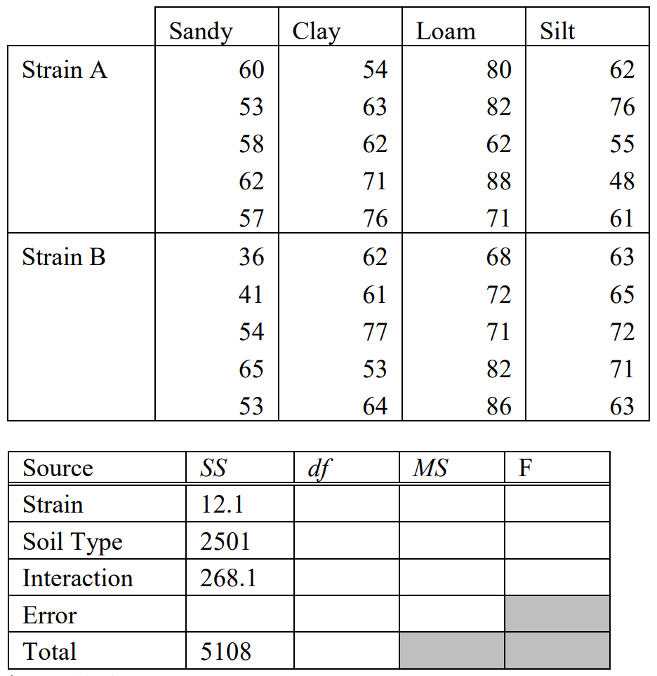
A farmer wants to see if there is a difference in the average height for two new strains of hemp plants. They believe there also may be some interaction with different soil types so they plant 5 hemp plants of each strain in 4 types of soil: sandy, clay, loam and silt. At \(\alpha\) = 0.01, analyze the data shown, using a two-way ANOVA as started below in Figure 11-6. See below for raw data.
.png?revision=1)
Solution
First, find the missing values for the ANOVA table in Figure 11-6. The sum of squares should add up to the total in the SS column of 5108.
Subtract the 3 sum of squares that were already given in the table from the total sum of squares to find the missing error sum of squares: \(5108 - 12.1 - 2501 - 268.1 = 2326.8\).
Find the degrees of freedom for each category.
There are 2 types of hemp strains so \(a = 2\) and the \(df_{\text{A}} = 2-1 = 1\).
There are 4 soil types so \(b = 4\) and the \(df_{\text{B}} = 4-1 = 3\).
The interaction \(df_{\text{A} \times \text{B}} = (2-1)(4-1) = 3\).
There are 5 plants within each group so \(n = 5\), and \(df_{\text{E}} = 2 \cdot 4(5-1) = 32\).
The total \(df\) should add up to \(N-1\). There are 8 groups of 5 so there are 40 data points all together; \(df_{\text{Total}} = 39\). Fill in your \(SS\) and \(df\) to the ANOVA table and then divide the sum of squares by \(df\) to get the mean squares. See below.
.png?revision=1)
Next, find the test statistic for by dividing the \(MS\) for each category by the \(MSE\). For the row effect \(F_{\text{A}} = 12.1/72.7125 = 0.1664\); for the column effect \(F_{\text{B}} = 833.6667/72.7125 = 11.4652\); and for the interaction effect \(F_{\text{A} \times \text{B}} = 89.3667/72/7125 = 1.2290\). Add these to complete the ANOVA table.
.png?revision=1)
There are three hypothesis tests that we are performing: the strain of hemp plan has an effect on the mean plant height (row effect), the type of soil has an effect on the mean plant height (column effect), and the interaction effect between strain of hemp plan and soil type on the mean plant height.
Row Effect-Factor A:
\(H_{0}:\) The strain of hemp plant has no effect on the mean plant height.
\(H_{1}:\) The strain of hemp plant has an effect on the mean plant height.
Test Statistic: \(F_{\text{A}} = 0.1664\).
Critical Value: Use an F-distribution with \(\alpha = 0.01\) right-tail area, \(df_{\text{A}} = 1\) and \(df_{\text{E}} = 32\).
The critical value is 7.4993. See Figure 11-7.
.png?revision=1)
The test statistic of 0.1664 is less than the critical value and not in the shaded tail; therefore, do not reject \(H_{0}\). There is no significant difference in the mean plant height between the two hemp strains.
Column Effect-Factor B:
\(H_{0}:\) The type of soil has no effect on the mean plant height.
\(H_{1}:\) The type of soil has an effect on the mean plant height.
Test Statistic: \(F_{\text{B}} = 11.4652\)
Critical Value: Use an F-distribution with \(\alpha\) = 0.01 right-tail area, \(df_{\text{B}} = 3\) and \(df_{\text{E}} = 32\). The critical value is 4.4594.
.png?revision=1)
The test statistic is greater than the critical value and is in the shaded tail; therefore, reject \(H_{0}\). The type of soil has a significant effect on the mean plant height.
Interaction Effect-Factor A \(\times\) B
\(H_{0}:\) There is no interaction effect between the strain of hemp and the soil type on the mean plant height.
\(H_{1}:\) There is an interaction effect between the strain of hemp and the soil type on the mean plant height.
Test Statistic: \(F_{\text{A} \times \text{B}} = 1.229\)
Critical Value: Use an F-distribution with \(\alpha\) = 0.01 right-tail area, \(df_{\text{A} \times \text{B}} = 3\) and \(df_{\text{E}} = 32\). The critical value is 4.4594.
.png?revision=1)
The test statistic is not in the shaded tail; therefore, do not reject \(H_{0}\). There is no significant interaction effect between the hemp strain and the soil type on the mean plant height.
Rough drawings from memory were futile. He didn't even know how long it had been, beyond Ford Prefect's rough guess at the time that it was "a couple of million years" and he simply didn't have the maths. Still, in the end he worked out a method which would at least produce a result. He decided not to mind the fact that with the extraordinary jumble of rules of thumb, wild approximations and arcane guesswork he was using he would be lucky to hit the right galaxy, he just went ahead and got a result. He would call it the right result. Who would know?
As it happened, through the myriad and unfathomable chances of fate, he got it exactly right, though he of course would never know that. He just went up to London and knocked on the appropriate door. "Oh. I thought you were going to phone me first."
(Adams, 2002)