
11.5: Chapter 11 Exercises
- Page ID
- 34780

1. What does the acronym ANOVA stand for?
a) Analysis of Variance
b) Analysis of Means
c) Analyzing Various Means
d) Analysis of Variance
e) Anticipatory Nausea and Vomiting
f) Average Noise Variance
2. What would the test statistic equal if MSB = MSW?
a) -1
b) 0
c) 1
d) 4
e) 1.96
3. A researcher would like to test to see if there is a difference in the average profit between 5 different stores. Which are the correct hypotheses for an ANOVA?
a) \(H_{0}: \mu_{1} = \mu_{2} = \mu_{3}\) \(H_{1}:\) At least one mean is different.
b) \(H_{0}: \mu_{1} = \mu_{2} = \mu_{3} = \mu_{4} = \mu_{5}\) \(H_{1}: \mu_{1} \neq \mu_{2} \neq \mu_{3} \neq \mu_{4} \neq \mu_{5}\)
c) \(H_{0}: \mu_{1} \neq \mu_{2} \neq \mu_{3} \neq \mu_{4} \neq \mu_{5}\) \(H_{1}: \mu_{1} = \mu_{2} = \mu_{3} = \mu_{4} = \mu_{5}\)
d) \(H_{0}: \sigma_{B}^{2} \neq \sigma_{W}^{2}\) \(H_{1}: \sigma_{B}^{2} = \sigma_{W}^{2}\)
e) \(H_{0}: \mu_{1} = \mu_{2} = \mu_{3} = \mu_{4} = \mu_{5}\) \(H_{1}:\) At least one mean is different
4. An ANOVA was run to test to see if there was a significant difference in the average cost between three different brands of snow skis. Random samples for each of the three brands were collected from different stores. Assume the costs are normally distributed. At \(\alpha\) = 0.05, test to see if there is a difference in the means. State the hypotheses, fill in the ANOVA table to find the test statistic, compute the p-value, state the decision and summary.
.png?revision=1)
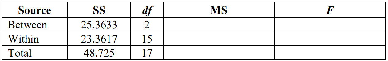
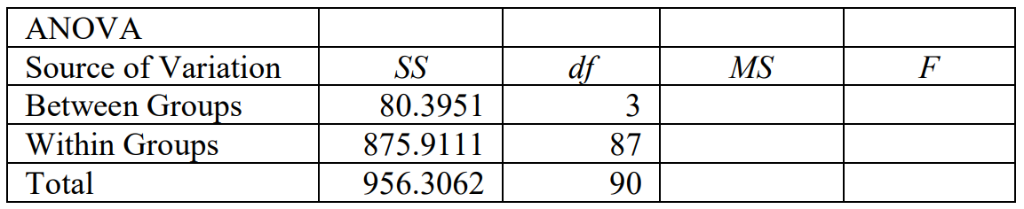
5. An ANOVA test was run for the per-pupil costs for private school tuition for three counties in the Portland, Oregon, metro area. Assume tuition costs are normally distributed. At \(\alpha\) = 0.05, test to see if there is a difference in the means.
.png?revision=1)
a) State the hypotheses.
b) Fill out the ANOVA table to find the test statistic.
.png?revision=1)
c) Compute the p-value.
d) State the correct decision and summary.
6. Cancer is a terrible disease. Surviving may depend on the type of cancer the person has. To see if the mean survival time for several types of cancer are different, data was collected on the survival time in days of patients with one of these cancers in advanced stage. The data is from "Cancer survival story," 2013. (Please realize that this data is from 1978. There have been many advances in cancer treatment, so do not use this data as an indication of survival rates from these cancers.) Does the data indicate that there is a difference in the mean survival time for these types of cancer? Use a 1% significance level.
.png?revision=1)
a) State the hypotheses.
b) Fill in an ANOVA table to find the test statistic.
c) Compute the p-value.
d) State the correct decision and summary.
7. What does the Bonferroni comparison test for?
a) The analysis of between and within variance.
b) The difference between all the means at once.
c) The difference between two pairs of mean.
d) The sample size between the groups.
8. True or false: The Bonferroni test should only be done when you reject the null hypothesis F-test?
9. A manufacturing company wants to see if there is a significant difference in three types of plastic for a new product. They randomly sample prices for each of the three types of plastic and run an ANOVA. Use \(\alpha\) = 0.05 to see if there is a statistically significant difference in the mean prices. Part of the computer output is shown below.
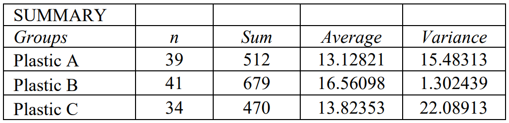.png?revision=1)
a) State the hypotheses.
b) Fill in the ANOVA table to find the test statistic.
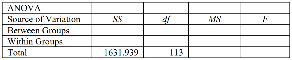.png?revision=1)
c) Compute the critical value.
d) State the decision and summary.
e) Which group(s) are significantly different based on the Bonferroni test?
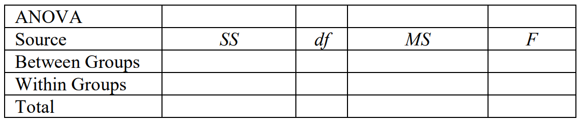
10. A manager on an assembly line wants to see if they can speed up production by implementing a new switch for their conveyor belts. There are four switches to choose from and replacing all the switches along the assembly line will be quite costly. They test out each of the four designs and record assembly times. Use \(\alpha\) = 0.05 to see if there is a statistically significant difference in the mean times.
.png?revision=1)
a) State the hypotheses.
b) Fill in the ANOVA table to find the test statistic.
c) Compute the critical value.
d) State the correct decision and summary.
e) Should a post-hoc Bonferroni test be done? Why?
i. No, since the p-value > \(\alpha\) there is no difference in the means.
ii. Yes, we should always perform a post-hoc test after an ANOVA
iii. No, since we already know that there is a difference in the means.
iv. Yes, since the p-value < \(\alpha\) we need to see where the differences are.
f) All four new switches are significantly faster than the current switch method. Of the four new types of switches, switch 3 cost the least amount to implement. Which of the 4, if any, should the manager choose?
i. The manager should stay with the old switch method since we failed to reject the null hypothesis.
ii. The manager should switch to any of the four new switches since we rejected the null hypothesis.
iii. The manager should randomly pick from switch types 1, 2 or 4.
iv. Since there is no statistically significant difference in the mean time they should choose switch 3 since it is the least expensive.
For exercises 11-16, Assume that all distributions are normal with equal population standard deviations, and the data was collected independently and randomly. Show all 5 steps for hypothesis testing. If there is a significant difference is found, run a Bonferroni test to see which means are different.
a) State the hypotheses.
b) Compute the test statistic.
c) Compute the critical value or p-value.
d) State the decision.
e) Write a summary.
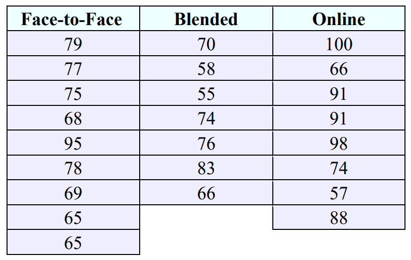
11. Is a statistics class's delivery type a factor in how well students do on the final exam? The table below shows the average percent on final exams from several randomly selected classes that used the different delivery types. Use a level of significance of \(\alpha\) = 0.10.
.png?revision=1)
12. The dependent variable is the number of times a photo gets a like on social media. The independent variable is the subject matter, selfie or people, landscape, meme, or a cute animal. The researcher is exploring whether the type of photo makes a difference on the mean number of likes. A random sample of photos were taken from social media. Test to see if there is a significant difference in the means using \(\alpha\) = 0.05.
.png?revision=1)
13. The dependent variable is movie ticket prices, and the groups are the geographical regions where the theaters are located (suburban, rural, urban). A random sample of ticket prices were taken from randomly chosen states. Test to see if there is a significant difference in the means using \(\alpha\) = 0.05.
.png?revision=1)
14. Recent research indicates that the effectiveness of antidepressant medication is directly related to the severity of the depression (Khan, Brodhead, Kolts & Brown, 2005). Based on pre-treatment depression scores, patients were divided into four groups based on their level of depression. After receiving the antidepressant medication, depression scores were measured again and the amount of improvement was recorded for each patient. The following data are similar to the results of the study. Use a significance level of \(\alpha\) = 0.05. Test to see if there is a difference in the mean scores.
.png?revision=1)
15. An ANOVA was run to test to see if there was a significant difference in the average cost between three different types of fabric for a new clothing company. Random samples for each of the three fabric types was collected from different manufacturers. At \(\alpha\) = 0.10, run an ANOVA test to see if there is a difference in the means.
.png?revision=1)
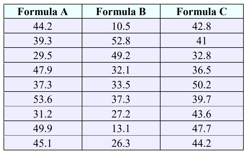
16. Three students, Linda, Tuan, and Javier, are given laboratory rats for a nutritional experiment. Each rat's weight is recorded in grams. Linda feeds her 9 rats Formula A, Tuan feeds his 9 rats Formula B, and Javier feeds his 9 rats Formula C. At the end of a specified time-period, each rat is weighed again, and the net gain in grams is recorded. Using a significance level of 0.10, test to see if there is a difference in the mean weight gain for the three formulas.
.png?revision=1)
17. For a two-way ANOVA, a row factor has 3 different levels, a column factor has 4 different levels. There are 15 data values in each group. Find the following.
a) The degrees of freedom for the row effect.
b) The degrees of freedom for the column effect.
c) The degrees of freedom for the interaction effect.
18. Fill out the following two-way ANOVA table.
.png?revision=1)
19. Fill out the following two-way ANOVA table.
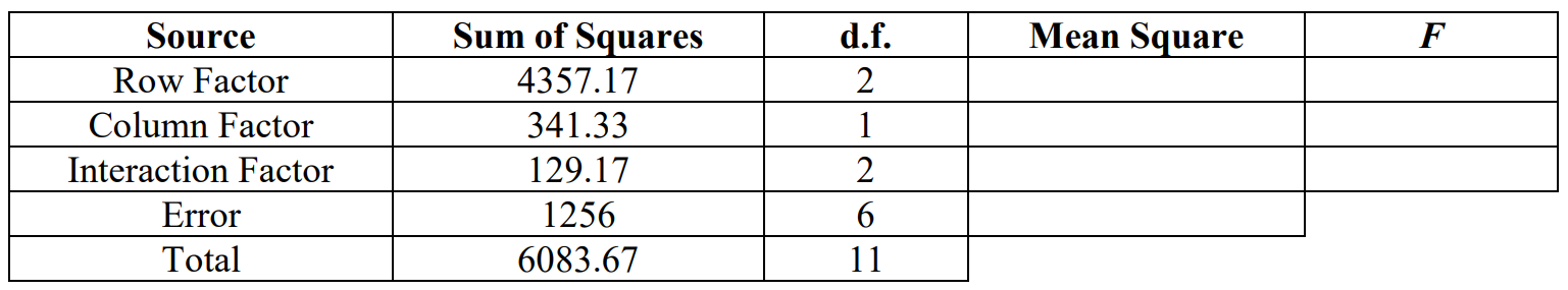.png?revision=1)
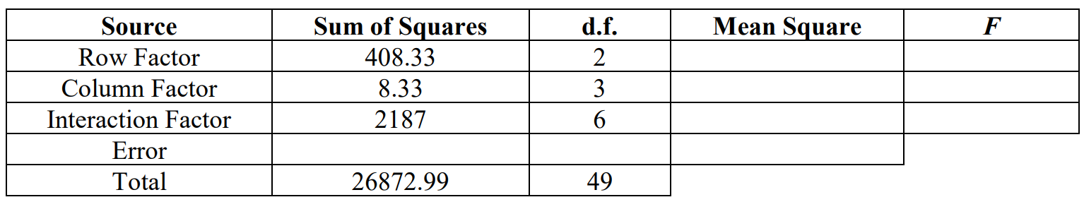
20. Fill out the following two-way ANOVA table.
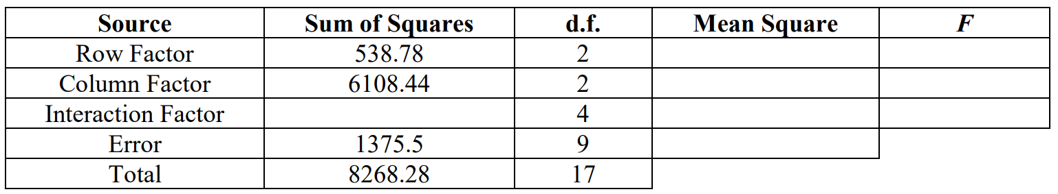.png?revision=1)
21. Fill out the following two-way ANOVA table.
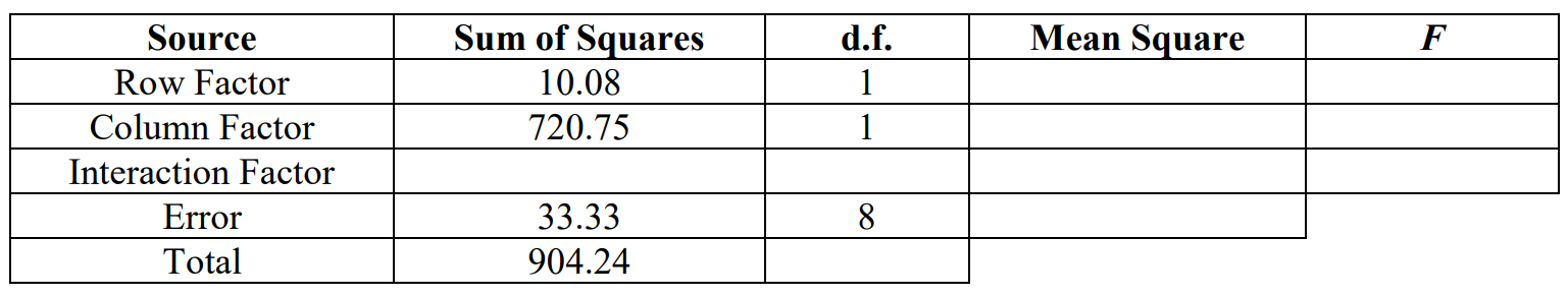.png?revision=1)
22. Fill out the following two-way ANOVA table.
.png?revision=1)
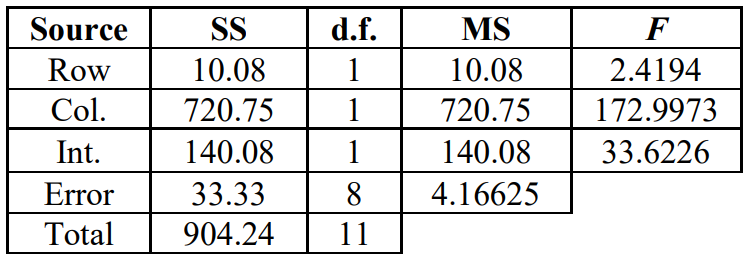
23. A professor is curious if class size and format for which homework is administered has an impact on students’ test grades. In a particular semester, she samples 4 students in each category below and records their grade on the department-wide final exam. The data are recorded below. Assume the variables are normally distributed. Run a two-way ANOVA using \(\alpha\) = 0.05.
.png?revision=1)
24. A study was conducted to observe the impact of young adults eating a diet that is high in healthy fats. A random sample of young adults was instructed to eat a particular menu for a month. They were then tested to check a combination of recall skills, reflexes, and physical fitness and scored from 1-10 based on performance. They were divided into two groups, one eating a menu that is high in healthy fats, and the other low in healthy fats. They were also divided based on age. The data are recorded below. Assume the variables are normally distributed. Run a two-way ANOVA using \(\alpha\) = 0.05.
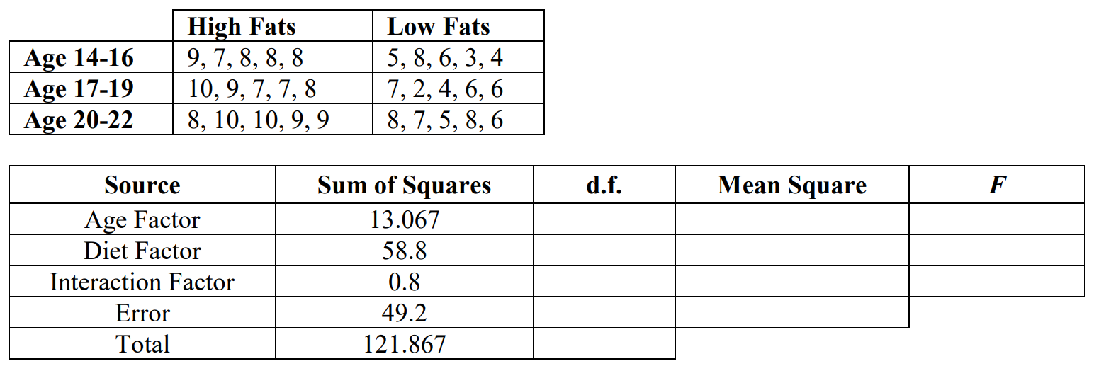.png?revision=1)
25. A door-to-door sales company sells three types of vacuums. The company manager is interested to find out if the type of vacuum sold has an effect on whether a sale is made, as well as what time of day the sale is made. She samples 36 sales representatives and divides them into the following categories, then records their sales (in hundreds of dollars) for a week. Assume the variables are normally distributed. Run a two-way ANOVA using \(\alpha\) = 0.05.
.png?revision=1)
26. A customer shopping for a used car is curious if the price of a vehicle varies based on type of vehicle and location of used car dealership. She samples 5 vehicles in each category below and records the price of each vehicle. Each vehicle is in similar shape in regards to age, mileage, and condition. A two-way ANOVA test was run and the information from the test is summarized in the table below. State all 3 hypotheses, critical values, decisions and summaries using \(\alpha\) = 0.05.
.png?revision=1)
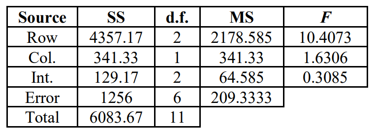
27. A sample of patients are tested for cholesterol level and divided into categories by age and by location of residence in the United States. The data are recorded below. Assume the variables are normally distributed. A two-way ANOVA test was run and the information from the test is summarized in the table below. State all 3 hypotheses, critical values, decisions and summaries using \(\alpha\) = 0.05.
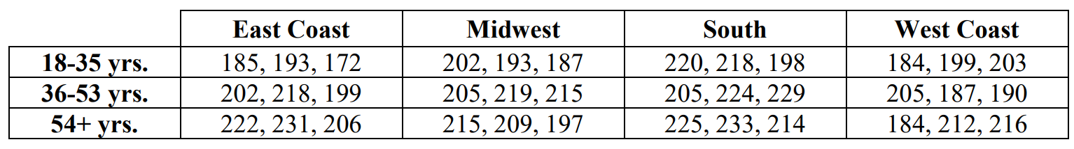.png?revision=1)
.png?revision=1)
28. The employees at a local nursery swear by a certain variety of tomato seed and a certain variety of fertilizer. To test their instincts, they take a sample of 3 varieties of tomato seed and 4 varieties of fertilizer and find the following yield of tomatoes from each tomato plant. Assume the variables are normally distributed. Run a two-way ANOVA using \(\alpha\) = 0.05.
.png?revision=1)
29. An obstetrician feels that her patients who are taller and leaner before becoming pregnant typically have quicker deliveries. She samples 3 women in each of the following categories of Height and Body Mass Index and records the time they spent in the pushing phase of labor in minutes. All women in the sample had a natural vaginal delivery and it was their first childbirth. The data are recorded below. Assume the variables are normally distributed. Run a two-way ANOVA using \(\alpha\) = 0.05.
.png?revision=1)
- Solutions to Odd-Numbered Exercises
-
1. a
3. e
5. \(H_{0}: \mu_{1} = \mu_{2} = \mu_{3}\); \(H_{1}:\) At least one mean is different.
F = 0.5902; p-value = 0.5605.
Do not reject \(H_{0}\). There is not enough evidence to support the claim that there is a difference in the mean per-pupil costs for private school tuition for three counties in the Portland, Oregon, metro area.7. c
9. a) \(H_{0}: \mu_{A} = \mu_{B} = \mu_{C}\); \(H_{1}:\) At least one mean is different.
b) \(F = 10.64046\)
c) \(F_{\alpha} = 3.0781\)
d) Reject \(H_{0}\). There is enough evidence to support the claim that there is a difference in the mean price of the three types of plastic.
e) \(H_{0}: \mu_{A} = \mu_{B}\); \(H_{1} = \mu_{A} \neq \mu_{B}\); p-value=0; reject \(H_{0}\). There is significant difference in price between plastics A and B. \(H_{0}: \mu_{A} = \mu_{C}\); \(H_{1} = \mu_{A} \neq \mu_{C}\); p-value = 1; do not reject \(H_{0}\). There is not a significant difference in price between plastics A and C. \(H_{0}: \mu_{B} = \mu_{C}\); \(H_{1} = \mu_{B} \neq \mu_{C}\); p-value = 0.003; reject \(H_{0}\). There is significant difference in price between plastics B and C.11. \(H_{0}: \mu_{1} = \mu_{2} = \mu_{3}\); \(H_{1}:\) At least one mean is different. F = 2.5459; p-value = 0.0904; do not reject \(H_{0}\). There is not enough evidence to support the claim that there is a difference in the mean movie ticket prices by geographical regions.
13. \(H_{0}: \mu_{1} = \mu_{2} = \mu_{3}\); \(H_{1}:\) At least one mean is different. F = 2.7121; p-value = 0.0896; reject \(H_{0}\). There is sufficient evidence to support the claim that course delivery type is a factor in final exam score.
15. \(H_{0}: \mu_{A} = \mu_{B} = \mu_{C}\); \(H_{1}:\) At least one mean is different. F = 2.895; p-value = 0.06; reject \(H_{0}\). 0. There is sufficient evidence to support the claim that there is a difference in the mean cost between three different types of fabric.
\(H_{0}: \mu_{A} = \mu_{B}\); \(H_{1}: \mu_{A} \neq \mu_{B}\); p-value = 1; do not reject \(H_{0}\). There is not a significant difference in the mean cost of fabrics A and B. \(H_{0}: \mu_{A} = \mu_{C}\); \(H_{1}: \mu_{A} \neq \mu_{C}\); p-value = 0.222; do not reject \(H_{0}\). There is not a significant difference in the mean cost of fabrics A and C. \(H_{0}: \mu_{B} = \mu_{C}\); \(H_{1}: \mu_{B} \neq \mu_{C}\); p-value = 0.07; reject \(H_{0}\). There is significant difference in the mean cost of fabrics B and C.17. a) \(df_{\text{A}} = 2, df_{\text{E}} = 168\)
b) \(df_{\text{B}} = 3, df_{\text{E}} = 168\)
c) \(df_{\text{A} \times \text{B}} = 6, df_{\text{E}} = 168\)19.
.png?revision=1)
21.
.png?revision=1)
23. \(H_{0}:\) The format of the homework (paper vs. online) has no effect on the mean test grade. \(H_{1}:\) The format of the homework (paper vs. online) has an effect on the mean test grade. F = 0.7185; CV = F.INV.RT(0.05,1,12) = 4.7472; do not reject \(H_{0}\). There is not enough evidence to support the claim that the format of the homework (paper vs. online) has an effect on the mean test grade.
\(H_{0}:\) The class size has no effect on the mean test grade. \(H_{1}:\) The class size has an effect on the mean test grade. F = 5.7064; CV = F.INV.RT(0.05,1,12) = 4.7472; reject \(H_{0}\). There is enough evidence to support the claim that the class size has an effect on the mean test grade.
\(H_{0}:\) There is no interaction effect between the format of the homework (paper vs. online) and the class size on the mean test grade. \(H_{1}:\) There is an interaction effect between the format of the homework (paper vs. online) and the class size on the mean test grade. F = 0.8082; CV = F.INV.RT(0.05,1,12) = 4.7472; do not reject \(H_{0}\). There is not enough evidence to support the claim that there is an interaction effect between the format of the homework (paper vs. online) and the class size on the mean test grade.25. \(H_{0}:\) The time of day has no effect on the mean number of vacuum sales. \(H_{1}:\) The time of day has an effect on the mean number of vacuum sales. F = 4.4179; CV = F.INV.RT(0.05,2,27) = 3.3541; reject \(H_{0}\). There is enough evidence to support the claim that the time of day has an effect on the mean number of vacuum sales.
\(H_{0}:\) The type of vacuum has no effect on the mean number of vacuum sales. \(H_{1}:\) The type of vacuum has an effect on the mean number of vacuum sales. F = 27.4172; CV = F.INV.RT(0.05,2,27) = 3.3541; reject \(H_{0}\). There is enough evidence to support the claim that the type of vacuum has an effect on the mean number of vacuum sales.
\(H_{0}:\) There is no interaction effect between time of day and type of vacuum on the mean number of vacuum sales. \(H_{1}:\) There is an interaction effect between time of day and type of vacuum on the mean number of vacuum sales. F = 0.9021; CV = F.INV.RT(0.05,4,27) = 2.7278; do not reject \(H_{0}\). There is not enough evidence to support the claim that there is an interaction effect between time of day and type of vacuum on the mean number of vacuum sales.27. \(H_{0}:\) Age has no effect on the mean cholesterol level. \(H_{1}:\) Age has an effect on the mean cholesterol level. F = 7.863; CV = F.INV.RT(0.05,2,24) = 3.4028; reject \(H_{0}\). There is enough evidence to support the claim that age has an effect on the mean cholesterol level.
\(H_{0}:\) Location has no effect on the mean cholesterol level. \(H_{1}:\) Location has no effect on the mean cholesterol level. F = 5.709; CV = F.INV.RT(0.05,3,24) = 3.0087; reject \(H_{0}\). There is enough evidence to support the claim that the location has an effect on the mean cholesterol level.
\(H_{0}:\) There is no interaction effect between age and location on the mean cholesterol level. \(H_{1}:\) There is an interaction effect between age and location on the mean cholesterol level. F = 1.455; CV = F.INV.RT(0.05,6,24) = 2.5082; do not reject \(H_{0}\). There is not enough evidence to support the claim that there is an interaction effect between age and location on the mean cholesterol level.29. \(H_{0}:\) Height has no effect on the mean delivery time. \(H_{1}:\) Height has an effect on the mean delivery time. F = 3.2798; CV = F.INV.RT(0.05,2,19) = 3.5219; do not reject \(H_{0}\). There is not enough evidence to support the claim that height has an effect on the mean delivery time.
\(H_{0}:\) BMI has no effect on the mean delivery time. \(H_{1}:\) BMI has an effect on the mean delivery time. F = 1.3763; CV = F.INV.RT(0.05,2,19) = 3.5219; do not reject \(H_{0}\). There is not enough evidence to support the claim that BMI has an effect on the mean delivery time.
\(H_{0}:\) There is no interaction effect between the height and BMI on the mean delivery time. \(H_{1}:\) There is an interaction effect between the height and BMI on the mean delivery time. F = 0.1125; CV = F.INV.RT(0.05,4,19) = 2.8951; do not reject \(H_{0}\). There is not enough evidence to support the claim that there is an interaction effect between the height and BMI on the mean delivery time.