7.7: t-Interval for a Mean

Last updated
Save as PDF

Page ID: 27483

$ \newcommand{\vecs}[1]{\overset { \scriptstyle \rightharpoonup} {\mathbf{#1}} } $ $ \newcommand{\vecd}[1]{\overset{-\!-\!\rightharpoonup}{\vphantom{a}\smash {#1}}} $$\newcommand{\id}{\mathrm{id}}$ $ \newcommand{\Span}{\mathrm{span}}$ $ \newcommand{\kernel}{\mathrm{null}\,}$ $ \newcommand{\range}{\mathrm{range}\,}$ $ \newcommand{\RealPart}{\mathrm{Re}}$ $ \newcommand{\ImaginaryPart}{\mathrm{Im}}$ $ \newcommand{\Argument}{\mathrm{Arg}}$ $ \newcommand{\norm}[1]{\| #1 \|}$ $ \newcommand{\inner}[2]{\langle #1, #2 \rangle}$ $ \newcommand{\Span}{\mathrm{span}}$ $\newcommand{\id}{\mathrm{id}}$ $ \newcommand{\Span}{\mathrm{span}}$ $ \newcommand{\kernel}{\mathrm{null}\,}$ $ \newcommand{\range}{\mathrm{range}\,}$ $ \newcommand{\RealPart}{\mathrm{Re}}$ $ \newcommand{\ImaginaryPart}{\mathrm{Im}}$ $ \newcommand{\Argument}{\mathrm{Arg}}$ $ \newcommand{\norm}[1]{\| #1 \|}$ $ \newcommand{\inner}[2]{\langle #1, #2 \rangle}$ $ \newcommand{\Span}{\mathrm{span}}$$\newcommand{\AA}{\unicode[.8,0]{x212B}}$

7.7.1 Student’s T-Distribution

A t-distribution is another symmetric distribution for a continuous random variable.

Gosset

William Gosset was a statistician employed at Guinness and performed statistics to find the best yield of barley for their beer. Guinness prohibited its employees to publish papers so Gosset published under the name Student. Gosset’s distribution is called the Student’s t-distribution.

A t-distribution is another special type of distribution for a continuous random variable.

Properties of the t-distribution density curve:

Symmetric, Unimodal (one mode) Bell-shaped.
Centered at the mean μ = median = mode = 0.
The spread of a t-distribution is determined by the degrees of freedom which are determined by the sample size.
As the degrees of freedom increase, the t-distribution approaches the standard normal curve.
The total area under the curve is equal to 1 or 100%.

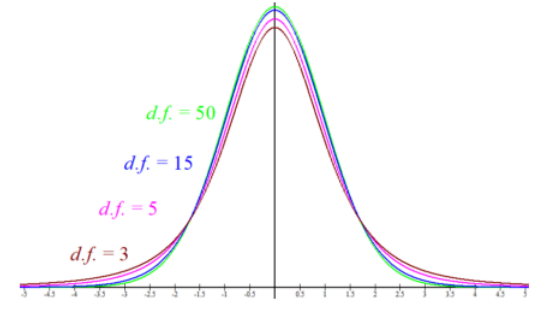
Figure 7-7

Figure 7-7 shows examples of three different t-distributions with degrees of freedom of 1, 5 and 30. Note that as the degrees of freedom increase the distribution has a smaller standard deviation and will get closer in shape to the normal distribution.

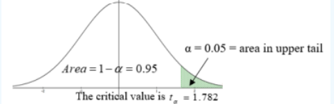
The t-critical value that has 5% of the area in the upper tail for n = 13.

Solution

Use a t-distribution with the degrees of freedom, df = n – 1 = 13 – 1 = 12. Draw and shade the upper tail area as in Figure 7-8. Use the DISTR menu invT option. Note that if you have an older TI-84 or a TI-83 calculator you need to have the program INVT installed.

For this function, you always use the area to the left of the point. If want 5% in the upper tail, then that means there is 95% in the bottom tail area. t_α = invT(area below t-score, df) = invT(0.95,12) = 1.782

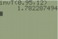
You can download the INVT program to your calculator from http://MostlyHarmlessStatistics.com or use Excel =T.INV(0.95,12) = 1.7823.

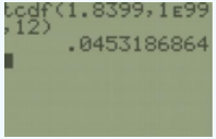
Compute the probability of getting a t-score larger than 1.8399 with a sample size of 13.

Solution

To find the P(t > 1.8399) on the TI calculator, go to DISTR use tcdf(lower,upper,df). For this example, we would have tcdf(1.8399,∞,12). In Excel use =1-T.DIST(1.8399,12,TRUE) = 0.0453. P(t > 1.8399) = 0.0453.

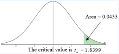
Figure 7-9

7.7.2 T-Confidence Interval

Note that we rarely have a calculation for the population standard deviation so in most cases we would need to use the sample standard deviation as an estimate for the population standard deviation. If we have a normally distributed population with an unknown population standard deviation then the sampling distribution of the sample mean will follow a t-distribution.

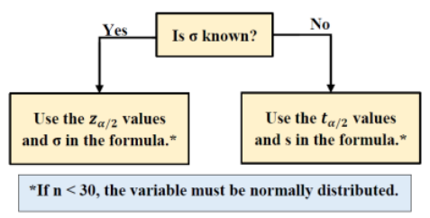
Figure 7-10

A 100(1 - $\alpha$)% Confidence Interval for a Population Mean μ: (σ unknown)

Choose a simple random sample of size n from a population having unknown mean μ.

The 100(1 - $\alpha$)% confidence interval estimate for μ is given by $\bar{x} \pm t_{\alpha / 2, n-1}\left(\frac{s}{\sqrt{n}}\right)$.

The df = degrees of freedom* are n – 1.

The degrees of freedom are the number of values that are free to vary after a sample statistic has been computed. For example, if you know the mean was 50 for a sample size of 4, you could pick any 3 numbers you like, but the 4^th value would have to be fixed to have the mean come out to be 50. For this class we just need to know that degrees of freedom will be based on the sample size.

The sample mean $\bar{x}$ is the point estimate for μ, and the margin of error is $t_{\alpha / 2}\left(\frac{s}{\sqrt{n}}\right)$. Where t_$\alpha$/2 is the positive critical value on the t-distribution curve with df = n – 1 and area 1 – $\alpha$ between the critical values –t_$\alpha$/2 and +t_$\alpha$/2, as shown in Figure 7-11.

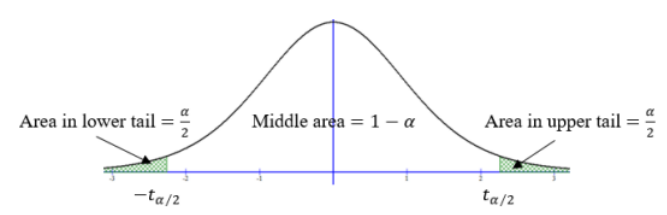
Figure 7-11

Before we compute a t-interval we will practice getting t critical values using Excel and the TI calculator’s built in tdistribution.

Compute the critical values –t_$\alpha$/2 and +t_$\alpha$/2 for a 90% confidence interval with a sample size of 10.

Solution

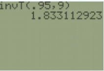
Draw and t-distribution with df = n – 1 = 9, see Figure 7-12. In Excel use =T.INV(lower tail area, df) =T.INV(0.95,9) or in the TI calculator use invT(lower tail area, df) = invT(0.95,9). The critical values are t = ±1.833

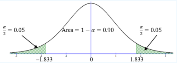
Figure 7-12

We can use Excel to find the margin of error when raw data is given in a problem. The following example is first done longhand and then done using Excel’s Data Analysis Tool and the T-Interval shortcut key on the TI calculator.

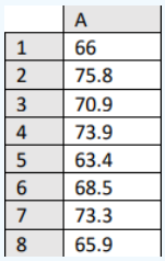
The yearly salary for mathematics assistant professors are normally distributed. A random sample of 8 math assistant professor’s salaries are listed below in thousands of dollars. Estimate the population mean salary with a 99% confidence interval.

66.0 75.8 70.9 73.9 63.4 68.5 73.3 65.9

Solution

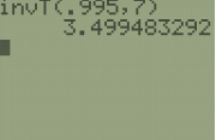
First find the t critical value using df = n – 1 = 7 and 99% confidence, t_$\alpha$/2 = 3.4995.

Then use technology to find the sample mean and sample standard deviation and substitute the numbers into the formula.

$\bar{x} \pm t_{\alpha / 2, n-1}\left(\frac{s}{\sqrt{n}}\right) \Rightarrow 69.7125 \pm 3.4995\left(\frac{4.4483}{\sqrt{8}}\right) \Rightarrow 69.7125 \pm 5.5037 \Rightarrow(64.2088,75.2162)$

The answer can be given as an inequality 64.2088 < µ < 75.2162 or in interval notation (64.2088, 75.2162).

We are 99% confident that the interval 64.2 and 75.2 contains the true population mean salary for all mathematics assistant professors.

We are 99% confident that the mean salary for mathematics assistant professors is between $64,208.80 and $75,216.20.

Assumption: The population we are sampling from must be normal* or approximately normal, and the population standard deviation σ is unknown. *This assumption must be addressed before using statistical inference for sample sizes of under 30.

TI-84: Press the [STAT] key, arrow over to the [TESTS] menu, arrow down to the [8:TInterval] option and press the [ENTER] key. Arrow over to the [Stats] menu and press the [ENTER] key. Then type in the mean, sample standard deviation, sample size and confidence level, arrow down to [Calculate] and press the [ENTER] key. The calculator returns the answer in interval notation. Be careful. If you accidentally use the [7:ZInterval] option you would get the wrong answer.

Alternatively (If you have raw data in list one) Arrow over to the [Data] menu and press the [ENTER] key. Then type in the list name, L₁, leave Freq:1 alone, enter the confidence level, arrow down to [Calculate] and press the [ENTER] key.

TI-89: Go to the [Apps] Stat/List Editor, then press [2^nd] then F7 [Ints], then select 2:TInterval. Choose the input method, data is when you have entered data into a list previously or stats when you are given the mean and standard deviation already. Type in the mean, standard deviation, sample size (or list name (list1), and Freq: 1) and confidence level, and press the [ENTER] key. The calculator returns the answer in interval notation. Be careful: If you accidentally use the [1:ZInterval] option you would get the wrong answer.

Excel Directions

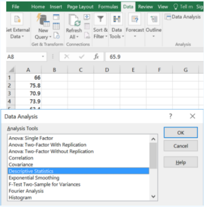
Type the data into Excel. Select the Data Analysis Tool under the Data tab.

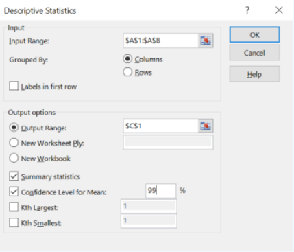
Select Descriptive Statistics. Select OK.

Use your mouse and click into the Input Range box, then select the cells containing the data. If you highlighted the label then check the box next to Labels in first row. In this case no label was typed in so the box is left blank. (Be very careful with this step. If you check the box and do not have a label then the first data point will become the label and all your descriptive statistics will be incorrect.)

Check the boxes next to Summary statistics and Confidence Level for Mean. Then change the confidence level to fit the question. Select OK.

The table output does not find the confidence interval. However, the output does give you the sample mean and margin of error.

The margin of error is the last entry labeled Confidence Level. To find the confidence interval subtract and add the margin of error to the sample mean to get the lower and upper limit of the interval in two separate cells.

The following screenshot shows the cell references to find the lower limit as =D3-D16 and the upper limit as =D3+D16. Make sure to put your answer in interval notation.

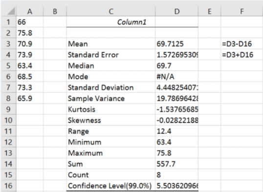
The answer is given as an inequality 64.2088 < µ < 75.2162 or in interval notation (64.2088, 75.2162).

We are 99% confident that the interval 64.2 and 75.2 contains the true population mean salary for all mathematics assistant professors.

Summary

A t-confidence interval is used to estimate an unknown value of the population mean for a single sample. We need to make sure that the population is normally distributed or the sample size is 30 or larger. Once this is verified we use the interval $\bar{x}-t_{\alpha / 2, n-1}\left(\frac{s}{\sqrt{n}}\right)<\mu<\bar{x}+t_{\alpha / 2, n-1}\left(\frac{s}{\sqrt{n}}\right)$ to estimate the true population mean. Most of the time we will be using the t-interval, not the z-interval, when estimating a mean since we rarely know the population standard deviation. It is important to interpret the confidence interval correctly. A general interpretation where you would change what is in the parentheses to fit the context of the problem is: “One can be 100(1 – $\alpha$)% confident that between (lower boundary) and (upper boundary) contains the population mean of (random variable in words using context and units from problem).”