7.2: Confidence Interval for a Proportion

Last updated
Save as PDF

Page ID: 24050

\( \newcommand{\vecs}[1]{\overset { \scriptstyle \rightharpoonup} {\mathbf{#1}} } \) \( \newcommand{\vecd}[1]{\overset{-\!-\!\rightharpoonup}{\vphantom{a}\smash {#1}}} \)\(\newcommand{\id}{\mathrm{id}}\) \( \newcommand{\Span}{\mathrm{span}}\) \( \newcommand{\kernel}{\mathrm{null}\,}\) \( \newcommand{\range}{\mathrm{range}\,}\) \( \newcommand{\RealPart}{\mathrm{Re}}\) \( \newcommand{\ImaginaryPart}{\mathrm{Im}}\) \( \newcommand{\Argument}{\mathrm{Arg}}\) \( \newcommand{\norm}[1]{\| #1 \|}\) \( \newcommand{\inner}[2]{\langle #1, #2 \rangle}\) \( \newcommand{\Span}{\mathrm{span}}\) \(\newcommand{\id}{\mathrm{id}}\) \( \newcommand{\Span}{\mathrm{span}}\) \( \newcommand{\kernel}{\mathrm{null}\,}\) \( \newcommand{\range}{\mathrm{range}\,}\) \( \newcommand{\RealPart}{\mathrm{Re}}\) \( \newcommand{\ImaginaryPart}{\mathrm{Im}}\) \( \newcommand{\Argument}{\mathrm{Arg}}\) \( \newcommand{\norm}[1]{\| #1 \|}\) \( \newcommand{\inner}[2]{\langle #1, #2 \rangle}\) \( \newcommand{\Span}{\mathrm{span}}\)\(\newcommand{\AA}{\unicode[.8,0]{x212B}}\)

Suppose you want to estimate the population proportion, p. As an example, an administrator may want to know what proportion of students at your school smoke. An insurance company may want to know what proportion of accidents are caused by teenage drivers who do not have a drivers’ education class. Every time we collect data from a new sample, we would expect the estimate of the proportion to change slightly. If you were to find a range of values over an interval this would give a better estimate of where the population proportion falls. This range of values that would better predict the true population parameter is called an interval estimate or confidence interval.

The sample proportion \(\hat{p}\) is the point estimate for p, the standard error (the standard deviation of the sampling distribution) of \(\hat{p}\) is \(\sqrt{\left(\frac{\hat{p} \cdot \hat{q}}{n}\right)}\), the z_α_/2is the critical value using the standard normal distribution, and the margin of error \(\mathrm{E}=Z_{\alpha / 2} \sqrt{\left(\frac{\hat{p} \cdot \hat{q}}{n}\right)}\). Some textbooks use \(\pi\) instead of p for the population proportion, and \(\bar{p}\) (pronounced “p-bar”) instead of \(\hat{p}\) for sample proportion.

Choose a simple random sample of size n from a population having unknown population proportion p. The 100(1 – \(\alpha\))% confidence interval estimate for p is given by \(\hat{p} \pm Z_{\alpha / 2} \sqrt{\left(\frac{\hat{p} \hat{q}}{n}\right)}\).

Where \(\hat{p}=\frac{x}{n}=\frac{\# \text { of successes }}{\# \text { of trials }}\) (read as “p hat”) is the sample proportion, and \(\hat{q}=1-\hat{p}\) is the complement.

The above confidence interval can be expressed as an inequality or an interval of values.

\(\hat{p}-z_{\alpha / 2} \sqrt{\left(\frac{\hat{p} \hat{q}}{n}\right)}<p<\hat{p}+z_{\alpha / 2} \sqrt{\left(\frac{\hat{p} \hat{q}}{n}\right)} \quad \text { or } \quad\left(\hat{p}-z_{\frac{\alpha}{2}} \sqrt{\left(\frac{\hat{p} \hat{q}}{n}\right)}, \hat{p}+z_{\alpha / 2} \sqrt{\left(\frac{\hat{p} \hat{q}}{n}\right)}\right)\)

Assumption: \(n \cdot \hat{p} \geq 10 \text { and } n \cdot \hat{q} \geq 10\)

*This assumption must be addressed before using these statistical inferences.

This formula is derived from the normal approximation of the binomial distribution, therefore the same conditions for a binomial need to be met, namely a set sample size of independent trials, two outcomes that have the same probability for each trial.

Steps for Calculating a Confidence Interval

1. State the random variable and the parameter in words.

x = number of successes

p = proportion of successes

2. State and check the assumptions for confidence interval.

a. A simple random sample of size n is taken.

b. The conditions for the binomial distribution are satisfied.

c. To determine the sampling distribution of \(\hat{p}\), you need to show that \(n \cdot \hat{p} \geq 10 \text { and } n \cdot \hat{q} \geq 10\), where \(\hat{q}\) = 1 − \(\hat{p}\). If this requirement is true, then the sampling distribution of \(\hat{p}\) is well approximated by a normal curve. (In reality, this is not really true, since the correct assumption deals with p. However, in a confidence interval you do not know p, so you must use \(\hat{p}\). This means you just need to show that x ≥ 10 and n – x ≥ 10.)

3. Compute the sample statistic \(\hat{p}=\frac{x}{n}\) and the confidence interval \(\hat{p} \pm z_\frac{\alpha}{2} \sqrt{\left(\frac{\hat{p} \hat{q}}{n}\right)}\).

4. Statistical Interpretation: In general, this looks like:

“We can be (1 – α)*100% confident that the interval \[\hat{p}-z_\frac{\alpha}{2} \sqrt{\left(\frac{\hat{p} \hat{q}}{n}\right)}<p<\hat{p}+z_\frac{\alpha}{2} \sqrt{\left(\frac{\hat{p} \hat{q}}{n}\right)}\]

Real World Interpretation: This is where you state what interval contains the true proportion.

A concern was raised in Australia that the percentage of deaths of indigenous Australian prisoners was higher than the percent of deaths of nonindigenous Australian prisoners, which is 0.27%. A sample of six years (1990- 1995) of data was collected, and it was found that out of 14,495 indigenous Australian prisoners, 51 died (“Indigenous deaths in,” 1996). Find a 95% confidence interval for the proportion of indigenous Australian prisoners who died.

Solution

1. State the random variable and the parameter in words.

x = number of indigenous Australian prisoners who die

p = proportion of indigenous Australian prisoners who die

2. State and check the assumptions for a confidence interval.

a. A simple random sample of 14,495 indigenous Australian prisoners was taken. However, the sample was not a random sample, since it was data from six years. It is the numbers for all prisoners in these six years, but the six years were not picked at random. Unless there was something special about the six years that were chosen, the sample is probably a representative sample. This assumption is probably met.

b. There are 14,495 prisoners in this case. The prisoners are all indigenous Australians, so you are not mixing indigenous Australian with nonindigenous Australian prisoners. There are only two outcomes, the prisoner either dies or does not. The chance that one prisoner dies over another may not be constant, but if you consider all prisoners the same, then it may be close to the same probability. Thus, the assumptions for the binomial distribution are satisfied.

c. In this case, x = 51 and n – x = 14,495 – 51 = 14,444. Both are greater than or equal to 10. The sampling distribution for \(\hat{p}\) is a normal distribution.

3. Compute the sample statistic and the confidence interval.

Sample Proportion: \(\hat{p}=\frac{x}{n}=\frac{51}{14495}=.003518\),

Critical Value: \(z_{\alpha / 2}=1.96\), since 95% confidence level

Margin of Error \(\mathrm{E}=z_{\alpha / 2} \sqrt{\left(\frac{\hat{p} \cdot \hat{q}}{n}\right)}=1.96 \sqrt{\left(\frac{0.003518(1-0.003518)}{14495}\right)}=0.000964\)

Confidence Interval: \(\hat{p}-\mathrm{E}<p<\hat{p}+\mathrm{E}\)

0.003518 – 0.000964 < p < 0.003518 + 0.000964

0.002554 < p < 0.004482 or (0.002554, 0.004482)

4. Statistical Interpretation: We can be 95% confident that 0.002554 < p < 0.004482 contains the proportion of all indigenous Australian prisoners who died.

5. Real World Interpretation: We can be 95% confident that the percentage of all indigenous Australian prisoners who died is between 0.26% and 0.45%.

Using Technology

Excel has no built-in shortcut key for finding a confidence interval for a proportion, but if you type in the following formulas shown below you can make your own Excel calculator where you just change the highlighted cells and all the numbers below will update with the relevant information.

Type in the following be cognizant of cell reference numbers.

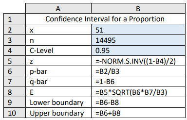
You get the following answers where the last two numbers are your confidence interval limits.

Make sure to put your answer in interval notation (0.002555, 0.004482) or 0.26% < p < 0.45%.

You can also do the calculations for the confidence interval with the TI Calculator.

TI-84: Press the [STAT] key, arrow over to the [TESTS] menu, arrow down to the [A:1-PropZInterval] option and press the [ENTER] key. Then type in the values for x, sample size and confidence level, arrow down to [Calculate] and press the [ENTER] key. The calculator returns the answer in interval notation. Note: Sometimes you are not given the x value but a percentage instead. To find the x to use in the calculator, multiply \(\hat{p}\) by the sample size and round off to the nearest integer. The calculator will give you an error message if you put in a decimal for x or n. For example, if \(\hat{p}\) = 0.22 and n = 124 then 0.22*124 = 27.28, so use x = 27.

TI-89: Go to the [Apps] Stat/List Editor, then press [2^nd] then F7 [Ints], then select 5: 1-PropZInt. Type in the values for x, sample size and confidence level, and press the [ENTER] key. The calculator returns the answer in interval notation. Note: sometimes you are not given the x value but a percentage instead. To find the x value to use in the calculator, multiply \(\hat{p}\) by the sample size and round off to the nearest integer. The calculator will give you an error message if you put in a decimal for x or n. For example, if \(\hat{p}\)= 0.22 and n = 124 then 0.22*124 = 27.28, so use x = 27.

A researcher studying the effects of income levels on new mothers breastfeeding their infants hypothesizes that those countries where the income level is lower has a higher rate of infants breastfeeding than higher income countries. It is known that in Germany, considered a high-income country by the World Bank, 22% of all babies are breastfed. In Tajikistan, considered a low-income country by the World Bank, researchers found that in a random sample of 500 new mothers that 125 were breastfeeding their infants. Find a 90% confidence interval of the proportion of mothers in low-income countries who breastfeed their infants.

Solution

1. State your random variable and the parameter in words.

x = The number of new mothers who breastfeed in a low-income country.

p = The proportion of new mothers who breastfeed in a low-income country.

2. State and check the assumptions for a confidence interval.

a. A simple random sample of 500 breastfeeding habits of new mothers in a low-income country was taken as was stated in the problem.

b. There were 500 women in the study. The women are considered identical, though they probably have some differences. There are only two outcomes - either the woman breastfeeds her baby or she does not. The probability of a woman breastfeeding her baby is probably not the same for each woman, but it is probably not that different for each woman. The assumptions for the binomial distribution are satisfied.

c. x = 125 and n – x = 500 – 125 = 375 and both are greater than or equal to 10, so the sampling distribution of \(\hat{p}\) is well approximated by a normal curve.

3. Compute the sample statistic and the confidence interval. On the TI-83/84: Go into the STAT menu. Move over to TESTS and choose 1- PropZInt, then press Calculate.

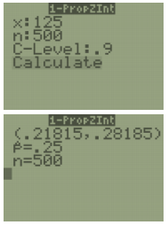
4. Statistical Interpretation: We are 90% confident that the interval 0.219 < p < 0.282 contains the population proportion of all women in low-income countries who breastfeed their infants.

5. Real World Interpretation: The proportion of women in low-income countries who breastfeed their infants is between 0.219 and 0.282 with 90% confidence.