
3.5: Chapter 3 Exercises
- Page ID
- 25882

1. A sample of eight cats found the following weights in kg.

a) Compute the mode.
b) Compute the median.
c) Compute the mean.
2. Cholesterol levels in milligrams (mg) of cholesterol per deciliter (dL) of blood, were collected from patients two days after they had a heart attack (Ryan, Joiner & Ryan, Jr, 1985).

Retrieved from http://www.statsci.org/data/general/cholest.html.
a) Compute the mode.
b) Compute the median.
c) Compute the mean.
3. The lengths (in kilometers) of rivers on the South Island of New Zealand that flow to the Tasman Sea are listed below.

Data from http://www.statsci.org/data/oz/nzrivers.html.
a) Compute the mode.
b) Compute the median.
c) Compute the mean.
4. A university assigns letter grades with the following 4-point scale: A = 4.00, A– = 3.67, B+ = 3.33, B = 3.00, B– = 2.67, C+ = 2.33, C = 2.00, C– = 1.67, D+ = 1.33, D = 1.00, D– = 0.67, F = 0.00. Calculate the grade point average (GPA) for a student who took in one term a 4 credit math course and received a B+, a 1 credit seminar course and received an A, a 3 credit history course and received an A- and a 5 credit writing course and received a D.
5. A university assigns letter grades with the following 4-point scale: A = 4.00, A– = 3.67, B+ = 3.33, B = 3.00, B– = 2.67, C+ = 2.33, C = 2.00, C– = 1.67, D+ = 1.33, D = 1.00, D– = 0.67, F = 0.00. Calculate the grade point average (GPA) for a student who took in one term a 3 credit biology course and received a C+, a 1 credit lab course and received a B, a 4 credit engineering course and received an A- and a 4 credit chemistry course and received a C+.
6. An employee at Clackamas Community College (CCC) is evaluated based on goal setting and accomplishments toward the goals, job effectiveness, competencies, and CCC core values. Suppose for a specific employee, goal 1 has a weight of 30%, goal 2 has a weight of 20%, job effectiveness has a weight of 25%, competency 1 has a weight of 4%, competency 2 has weight of 3%, competency 3 has a weight of 3%, competency 4 has a weight of 3%, competency 5 has a weight of 2%, and core values has a weight of 10%. Suppose the employee has scores of 3.0 for goal 1, 3.0 for goal 2, 2.0 for job effectiveness, 3.0 for competency 1, 2.0 for competency 2, 2.0 for competency 3, 3.0 for competency 4, 4.0 for competency 5, and 3.0 for core values. Compute the weighted mean score for this employee. If an employee has a score less than 2.5, they must have a Performance Enhancement Plan written. Does this employee need a plan?
7. A statistics class has the following activities and weights for determining a grade in the course: test 1 worth 15% of the grade, test 2 worth 15% of the grade, test 3 worth 15% of the grade, homework worth 10% of the grade, semester project worth 20% of the grade, and the final exam worth 25% of the grade. If a student receives an 85 on test 1, a 76 on test 2, an 83 on test 3, a 74 on the homework, a 65 on the project, and a 61 on the final, what grade did the student earn in the course? All the assignments were out of 100 points.
8. A statistics class has the following activities and weights for determining a grade in the course: test 1 worth 15% of the grade, test 2 worth 15% of the grade, test 3 worth 15% of the grade, homework worth 10% of the grade, semester project worth 20% of the grade, and the final exam worth 25% of the grade. If a student receives a 25 out of 30 on test 1, a 20 out of 30 on test 2, a 28 out of 30 on test 3, a 120 out of 140 points on the homework, a 65 out of 100 on the project, and a 31 out of 35 on the final, what grade did the student earn in the course?
9. A sample of eight cats found the following weights in kg.

a) Compute the range.
b) Compute the variance.
c) Compute the standard deviation.
10. The following data represents the percent change in tuition levels at public, four-year colleges (inflation adjusted) from 2008 to 2013 (Weissmann, 2013). To the right is the histogram. What is the shape of the distribution?

11. The following is a histogram of quiz grades.

a) What is the shape of the distribution?
b) Which is higher, the mean or the median?
12. Cholesterol levels were collected from patients two days after they had a heart attack (Ryan, Joiner & Ryan, Jr, 1985). Retrieved from http://www.statsci.org/data/general/cholest.html.

a) Compute the range.
b) Compute the variance.
c) Compute the standard deviation.
13. Suppose that a manager wants to test two new training programs. The manager randomly selects five people for each training type and measures the time it takes to complete a task after the training. The times for both trainings are in table below. Which training method is more variable?

14. The lengths (in kilometers) of rivers on the South Island of New Zealand that flow to the Tasman Sea are listed below.

Data from http://www.statsci.org/data/oz/nzrivers.html.
a) Compute the range.
b) Compute the variance.
c) Compute the standard deviation.
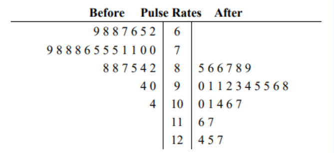
15. Here are pulse rates before and after exercise. Which group has the larger range?
16. A midterm in a statistics course had a mean score of 70 with a standard deviation 5. A quiz in a biology course had an average of 20 with a standard deviation of 5.
a) Compute the coefficient of variation for the statistics midterm exam.
b) Compute the coefficient of variation for the biology quiz.
c) Aaliyah scored a 75 on the statistics midterm exam. Compute Aaliyah’s z-score.
d) Viannie scored a 25 on the biology quiz. Compute Viannie’s z-score.
e) Which student did better on their respect test? Why? f) Was there more variability for the midterm or the quiz scores? Justify your answer with statistics.
17. The following is a sample of quiz scores.

a) Compute \(\overline{ x }\).
b) Compute s2.
c) Compute the median.
d) Compute the coefficient of variation.
e) Compute the range.
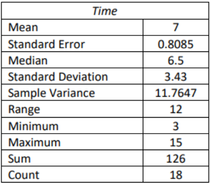
18. The time it takes to fill an online order was recorded and the following descriptive statistics were found using Excel. What is the coefficient of variation?
19. The following is the height and weight of a random sample of baseball players.

a) Compute the coefficient of variation for both height and weight.
b) Is there more variation in height or weight?a) Compute the coefficient of variation for both height and weight.
20. A midterm in a statistics course had a mean score of 70 with a standard deviation 5. A quiz had an average of 20 with a standard deviation of 5. A student scored a 73 on their midterm and 22 on their quiz. On which test did the student do better on compared to the rest of the class? Justify your answer with statistics.
21. The length of a human pregnancy is normally distributed with a mean of 272 days with a standard deviation of 9.1 days. William Hunnicut was born in Portland, Oregon, at just 181 days into his gestation. What is the zscore for William Hunnicut’s gestation? Retrieved from: http://digitalcommons.georgefox.edu/cgi/viewcontent.cgi?article=1149&context=gfc_life.
22. Arm span (sometimes referred to as wingspan) is the physical measurement of the length of an individual's arms from fingertip to fingertip. The average arm span of a man is 70 inches with a standard deviation of 4.5 inches. The Olympic gold medalists Michael Phelps has an arm span of 6 feet 7 inches, which is three inches more than his height. What is the z-score for Michael Phelps arm span?
23. The average time to run the Pikes Peak Marathon 2017 was 7.44 hours with a standard deviation of 1.34 hours. Rémi Bonnet won the Pikes Peak Marathon with a run time of 3.62 hours. Retrieved from: http://pikespeakmarathon.org/results/ppm/2017/.
The Tevis Cup 100-mile one-day horse race for 2017 had an average finish time of 20.38 hours with a standard deviation of 1.77 hours. Tennessee Lane won the 2017 Tevis cup in a ride time of 14.75 hours. Retrieved from: https://aerc.org/rpts/RideResults.aspx.
a) Compute the z-score for Rémi Bonnet’s time.
b) Compute the z-score for Tennessee Lane’s time.
c) Which competitor did better compared to their respective events?
24. Cholesterol levels were collected from patients two days after they had a heart attack (Ryan, Joiner & Ryan, Jr, 1985). Retrieved from http://www.statsci.org/data/general/cholest.html.
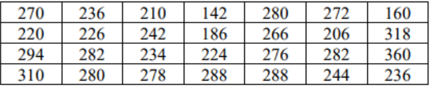
a) Compute the 25th percentile.
b) Compute the 90th percentile.
c) Compute the 5th percentile.
d) Compute Q3.
25. A sample of eight cats found the following weights in kg. Compute the 5-number summary.

26. The following data represent the grade point averages for a sample of 15 PSU students.

a) Compute the lower and upper limits.
b) Identify if there are any outliers.
c) Draw a modified box-and-whisker plot.
27. The lengths (in kilometers) of rivers on the South Island of New Zealand that flow to the Tasman Sea are listed below.

Data from http://www.statsci.org/data/oz/nzrivers.html.
a) Compute the 5-number summary.
b) Compute the lower and upper limits and any outlier(s) if any exist.
c) Make a modified box-and-whisker plot.
28. The following are box-and-whiskers plot for life expectancy for European countries and Southeast Asian countries from 2011. What is the distribution shape of the European countries’ life expectancy?

29. To determine if Reiki is an effective method for treating pain, a pilot study was carried out where a certified second-degree Reiki therapist provided treatment on volunteers. Pain was measured using a visual analogue scale (VAS) immediately before and after the Reiki treatment (Olson & Hanson, 1997). Higher numbers mean the patients had more pain.
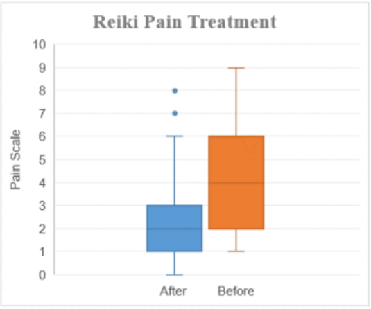
a) Use the box-and-whiskers plots to determine the IQR for the before treatment measurements.
b) Use the box-and-whiskers plots of the before and after VAS ratings to determine if the Reiki method was effective in reducing pain.
30. The median household income (in $1,000s) from a random sample of 100 counties that gained population over 2000-2010 are shown on the left. Median incomes from a random sample of 50 counties that had no population gain are shown on the right.

(OpenIntro Statistics, 2016)
What is the distribution shape for the counties with no population gain?
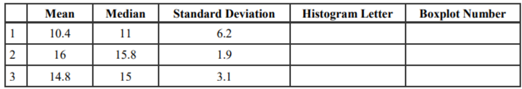
31. Match the correct descriptive statistics to the letter of the corresponding histogram and boxplot. Choose the correct letter for the corresponding histogram and Roman numeral for the corresponding boxplot. You should only use the visual representation, the definition of standard deviation and measures of central tendency to match the graphs with their respective descriptive statistics.
i. 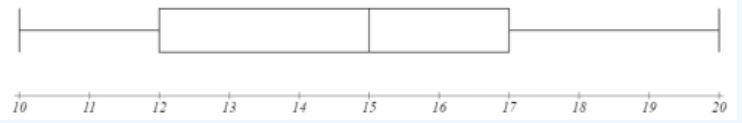
ii. 
iii. 
a) 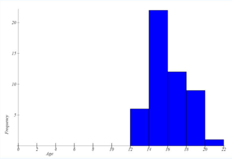
b)

c) 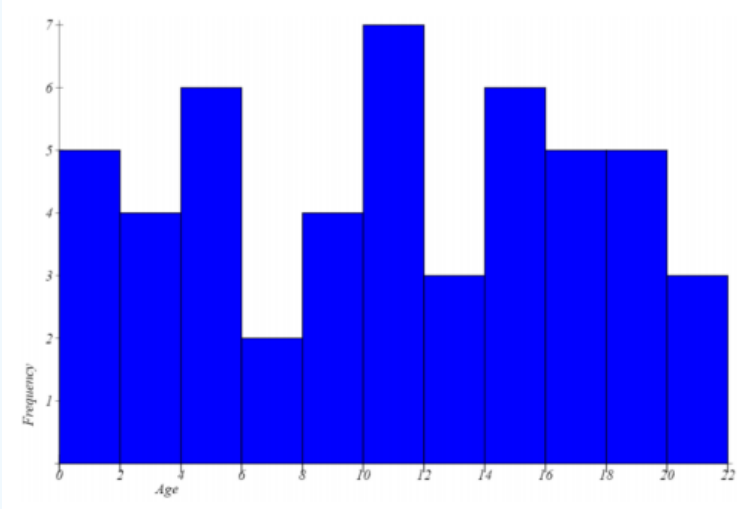
32. A sample has the following statistics: Minimum = 10, Maximum = 50, Range = 40, \(\overline{ x }\) = 20, mode = 32, Q1 =30, Q2 =35, Q3 =38, standard deviation = 5 and IQR = 8.
a) According to Chebyshev’s Inequality, what percentage of data would fall within the values 12.5 and 27.5?
b) If this sample were bell-shaped what percentage of the data would fall within the values 10 and 30?
33. The length of a human pregnancy is bell-shaped with a mean of 272 days with a standard deviation of 9 days (Bhat & Kushtagi, 2006). Compute the percentage of pregnancies that last between 245 and 299 days.
34. Arm span is the physical measurement of the length of an individual's arms from fingertip to fingertip. A man’s arm span is approximately bell-shaped with mean of 70 inches with a standard deviation of 4.5 inches. What percent of men have an arm span between 61 and 79 inches?
35. The size of fish is very important to commercial fishing. A study conducted in 2012 found the length of Atlantic cod caught in nets in Karlskrona to have a mean of 49.9 cm and a standard deviation of 3.74 cm (Ovegard, Berndt & Lunneryd, 2012).
a) According to Chebyshev’s Inequality, at least what percent of Atlantic cod should be between 44.29 and 55.51 cm?
b) Assume the length of Atlantic cod is bell-shaped. Approximately what percent of Atlantic cod are between 46.16 and 53.64 cm?
c) Assume the length of Atlantic cod is bell-shaped. Approximately what percent of Atlantic cod are between 42.42 and 57.38 cm?
36. Scores on the SAT for a certain year were bell-shaped with a mean of 1511 and a standard deviation of 194.
a) What two SAT scores that separated the middle 68% of SAT scores for that year?
b) What two SAT scores that separated the middle 95% of SAT scores for that year?
c) How high did a student need to score that year to be in the top 2.5%?
37. In a mid-size company, the distribution of the number of phone calls answered each day by each of the 12 employees is bell-shaped and has a mean of 59 and a standard deviation of 10. Using the empirical rule, what is the approximate percentage of daily phone calls numbering between 29 and 89?
38. The number of potholes in any given 1 mile stretch of pavement in Portland has a bell-shaped distribution. This distribution has a mean of 54 and a standard deviation of 5. Using the empirical rule, what is the approximate percentage of 1-mile long roadways with potholes numbering between 44 and 59?
39. A company has a policy of retiring company cars; this policy looks at number of miles driven, purpose of trips, style of car and other features. The distribution of the number of months in service for the fleet of cars is bellshaped and has a mean of 42 months and a standard deviation of 3 months. Using the Empirical Rule, what is the approximate percentage of cars that remain in service between 48 and 51 months?
40. The following is an infant weight percentile chart. What is the 50th percentile height in cm for a 10-month old boy?

Retrieved from: https://www.cdc.gov/growthcharts/data/set1clinical/cj41l017.pdf.
- Answer to Odd Numbered Exercises
-
1 a) mode = 4 b) median = 3.75 c) \(\overline{ x }\) = 3.725
3) a) 56 & 64 b) 64 c) 67.6818
5) 2.833
7) 72.25
9) a) Range = 0.9 b) s 2 = 0.0870 c) s = 0.2949
11) a) Negatively skewed b) The median is higher.
13) s1 = 9.9348, s2 = 3.3466; Training 1 is more variable
15) Before range = 42, after range = 42, both groups have the same range.
17) a) 30.35 b) 136.7 c) 32.7 d) 38.52% e) 28.4
19) a) CVheight = 3.04%; CVweight = 9.84% b) Weight, because it has a higher coefficient of variation.
21) -10
23) a) -2.8507 b) -3.1808 c) Tennessee Lane
25) Min = 3.2, Q1 = 3.45 (TI: 3.55), Q2 = 3.7, Q3 = 3.95 (TI: 3.85), Max = 4.1
27) a) Min = 32, Q1 = 46 (TI: 48), Q2 = 64, Q3 = 77 (TI: 76), Max = 177 b) lower limit = -0.5 (TI: 6), upper limit = 123.5 (TI: 118), outliers = 177 (TI: 121 & 177) c)

29) a) 4 b) Yes, the treatment was effective.
31) 1. c. ii; 2. a. iii; 3. b. i
33) 99.7%
35) a) 55.56% b) 68% c) 95%
37) 99.7%
39) 2.35%