
10.1: Linear Relationships Between Variables
- Page ID
- 541
\( \newcommand{\vecs}[1]{\overset { \scriptstyle \rightharpoonup} {\mathbf{#1}} } \)
\( \newcommand{\vecd}[1]{\overset{-\!-\!\rightharpoonup}{\vphantom{a}\smash {#1}}} \)
\( \newcommand{\id}{\mathrm{id}}\) \( \newcommand{\Span}{\mathrm{span}}\)
( \newcommand{\kernel}{\mathrm{null}\,}\) \( \newcommand{\range}{\mathrm{range}\,}\)
\( \newcommand{\RealPart}{\mathrm{Re}}\) \( \newcommand{\ImaginaryPart}{\mathrm{Im}}\)
\( \newcommand{\Argument}{\mathrm{Arg}}\) \( \newcommand{\norm}[1]{\| #1 \|}\)
\( \newcommand{\inner}[2]{\langle #1, #2 \rangle}\)
\( \newcommand{\Span}{\mathrm{span}}\)
\( \newcommand{\id}{\mathrm{id}}\)
\( \newcommand{\Span}{\mathrm{span}}\)
\( \newcommand{\kernel}{\mathrm{null}\,}\)
\( \newcommand{\range}{\mathrm{range}\,}\)
\( \newcommand{\RealPart}{\mathrm{Re}}\)
\( \newcommand{\ImaginaryPart}{\mathrm{Im}}\)
\( \newcommand{\Argument}{\mathrm{Arg}}\)
\( \newcommand{\norm}[1]{\| #1 \|}\)
\( \newcommand{\inner}[2]{\langle #1, #2 \rangle}\)
\( \newcommand{\Span}{\mathrm{span}}\) \( \newcommand{\AA}{\unicode[.8,0]{x212B}}\)
\( \newcommand{\vectorA}[1]{\vec{#1}} % arrow\)
\( \newcommand{\vectorAt}[1]{\vec{\text{#1}}} % arrow\)
\( \newcommand{\vectorB}[1]{\overset { \scriptstyle \rightharpoonup} {\mathbf{#1}} } \)
\( \newcommand{\vectorC}[1]{\textbf{#1}} \)
\( \newcommand{\vectorD}[1]{\overrightarrow{#1}} \)
\( \newcommand{\vectorDt}[1]{\overrightarrow{\text{#1}}} \)
\( \newcommand{\vectE}[1]{\overset{-\!-\!\rightharpoonup}{\vphantom{a}\smash{\mathbf {#1}}}} \)
\( \newcommand{\vecs}[1]{\overset { \scriptstyle \rightharpoonup} {\mathbf{#1}} } \)
\( \newcommand{\vecd}[1]{\overset{-\!-\!\rightharpoonup}{\vphantom{a}\smash {#1}}} \)
\(\newcommand{\avec}{\mathbf a}\) \(\newcommand{\bvec}{\mathbf b}\) \(\newcommand{\cvec}{\mathbf c}\) \(\newcommand{\dvec}{\mathbf d}\) \(\newcommand{\dtil}{\widetilde{\mathbf d}}\) \(\newcommand{\evec}{\mathbf e}\) \(\newcommand{\fvec}{\mathbf f}\) \(\newcommand{\nvec}{\mathbf n}\) \(\newcommand{\pvec}{\mathbf p}\) \(\newcommand{\qvec}{\mathbf q}\) \(\newcommand{\svec}{\mathbf s}\) \(\newcommand{\tvec}{\mathbf t}\) \(\newcommand{\uvec}{\mathbf u}\) \(\newcommand{\vvec}{\mathbf v}\) \(\newcommand{\wvec}{\mathbf w}\) \(\newcommand{\xvec}{\mathbf x}\) \(\newcommand{\yvec}{\mathbf y}\) \(\newcommand{\zvec}{\mathbf z}\) \(\newcommand{\rvec}{\mathbf r}\) \(\newcommand{\mvec}{\mathbf m}\) \(\newcommand{\zerovec}{\mathbf 0}\) \(\newcommand{\onevec}{\mathbf 1}\) \(\newcommand{\real}{\mathbb R}\) \(\newcommand{\twovec}[2]{\left[\begin{array}{r}#1 \\ #2 \end{array}\right]}\) \(\newcommand{\ctwovec}[2]{\left[\begin{array}{c}#1 \\ #2 \end{array}\right]}\) \(\newcommand{\threevec}[3]{\left[\begin{array}{r}#1 \\ #2 \\ #3 \end{array}\right]}\) \(\newcommand{\cthreevec}[3]{\left[\begin{array}{c}#1 \\ #2 \\ #3 \end{array}\right]}\) \(\newcommand{\fourvec}[4]{\left[\begin{array}{r}#1 \\ #2 \\ #3 \\ #4 \end{array}\right]}\) \(\newcommand{\cfourvec}[4]{\left[\begin{array}{c}#1 \\ #2 \\ #3 \\ #4 \end{array}\right]}\) \(\newcommand{\fivevec}[5]{\left[\begin{array}{r}#1 \\ #2 \\ #3 \\ #4 \\ #5 \\ \end{array}\right]}\) \(\newcommand{\cfivevec}[5]{\left[\begin{array}{c}#1 \\ #2 \\ #3 \\ #4 \\ #5 \\ \end{array}\right]}\) \(\newcommand{\mattwo}[4]{\left[\begin{array}{rr}#1 \amp #2 \\ #3 \amp #4 \\ \end{array}\right]}\) \(\newcommand{\laspan}[1]{\text{Span}\{#1\}}\) \(\newcommand{\bcal}{\cal B}\) \(\newcommand{\ccal}{\cal C}\) \(\newcommand{\scal}{\cal S}\) \(\newcommand{\wcal}{\cal W}\) \(\newcommand{\ecal}{\cal E}\) \(\newcommand{\coords}[2]{\left\{#1\right\}_{#2}}\) \(\newcommand{\gray}[1]{\color{gray}{#1}}\) \(\newcommand{\lgray}[1]{\color{lightgray}{#1}}\) \(\newcommand{\rank}{\operatorname{rank}}\) \(\newcommand{\row}{\text{Row}}\) \(\newcommand{\col}{\text{Col}}\) \(\renewcommand{\row}{\text{Row}}\) \(\newcommand{\nul}{\text{Nul}}\) \(\newcommand{\var}{\text{Var}}\) \(\newcommand{\corr}{\text{corr}}\) \(\newcommand{\len}[1]{\left|#1\right|}\) \(\newcommand{\bbar}{\overline{\bvec}}\) \(\newcommand{\bhat}{\widehat{\bvec}}\) \(\newcommand{\bperp}{\bvec^\perp}\) \(\newcommand{\xhat}{\widehat{\xvec}}\) \(\newcommand{\vhat}{\widehat{\vvec}}\) \(\newcommand{\uhat}{\widehat{\uvec}}\) \(\newcommand{\what}{\widehat{\wvec}}\) \(\newcommand{\Sighat}{\widehat{\Sigma}}\) \(\newcommand{\lt}{<}\) \(\newcommand{\gt}{>}\) \(\newcommand{\amp}{&}\) \(\definecolor{fillinmathshade}{gray}{0.9}\)To learn what it means for two variables to exhibit a relationship that is close to linear, but which contains an element of randomness
The following table gives examples of the kinds of pairs of variables which could be of interest from a statistical point of view.
| \(x\) | \(y\) |
|---|---|
| Predictor or independent variable | Response or dependent variable |
| Temperature in degrees Celsius | Temperature in degrees Fahrenheit |
| Area of a house (sq.ft.) | Value of the house |
| Age of a particular make and model car | Resale value of the car |
| Amount spent by a business on advertising in a year | Revenue received that year |
| Height of a \(25\)-year-old man | Weight of the man |
The first line in the table is different from all the rest because in that case and no other the relationship between the variables is deterministic: once the value of \(x\) is known the value of \(y\) is completely determined. In fact there is a formula for \(y\) in terms of \(x\):
\[y=95x+32 \nonumber \]
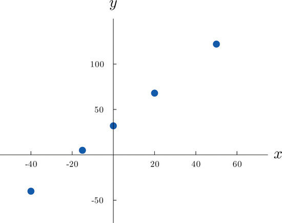
Choosing several values for \(x\) and computing the corresponding value for \(y\) for each one using the formula gives the table
\[\begin{array}{c|c c c c c} x & -40 & -15 & 0 & 20 & 50 \\ \hline y &-40 &5 &32 &68 &122\\ \end{array} \nonumber \]
We can plot these data by choosing a pair of perpendicular lines in the plane, called the coordinate axes, as shown in Figure \(\PageIndex{1}\). Then to each pair of numbers in the table we associate a unique point in the plane, the point that lies \(x\) units to the right of the vertical axis (to the left if \(x<0\)) and y units above the horizontal axis (below if \(y<0\)). The relationship between \(x\) and \(y\) is called a linear relationship because the points so plotted all lie on a single straight line. The number \(95\) in the equation \(y=95x+32\) is the slope of the line, and measures its steepness. It describes how y changes in response to a change in \(x\): if \(x\) increases by \(1\) unit then \(y\) increases (since \(95\) is positive) by \(95\) unit. If the slope had been negative then \(y\) would have decreased in response to an increase in \(x\). The number \(32\) in the formula \(y=95x+32\) is the \(y\)-intercept of the line; it identifies where the line crosses the \(y\)-axis. You may recall from an earlier course that every non-vertical line in the plane is described by an equation of the form \(y=mx+b\), where \(m\) is the slope of the line and \(b\) is its \(y\)-intercept.
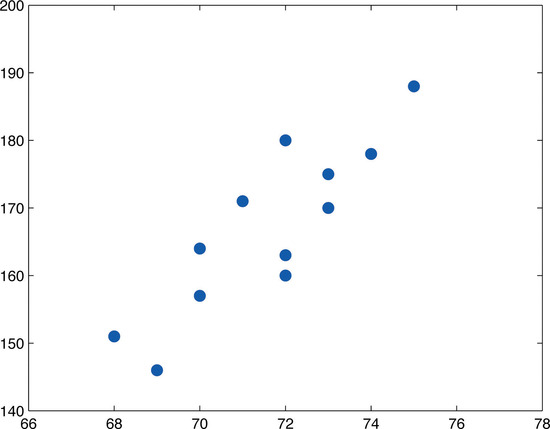
The relationship between \(x\) and \(y\) in the temperature example is deterministic because once the value of \(x\) is known, the value of \(y\) is completely determined. In contrast, all the other relationships listed in the table above have an element of randomness in them. Consider the relationship described in the last line of the table, the height \(x\) of a man aged \(25\) and his weight \(y\). If we were to randomly select several \(25\)-year-old men and measure the height and weight of each one, we might obtain a collection of \((x,y)\) pairs something like this:
\[(68,151)\; \; (72,163)\; \; (69,146)\; \; (72,180)\; \; (70,157)\; \; (73,170)\; \; (70,164)\; \; (73,175)\; \; (71,171)\; \; (74,178)\; \; (72,160)\; \; (75,188) \nonumber \]
A plot of these data is shown in Figure \(\PageIndex{2}\). Such a plot is called a scatter diagram or scatter plot. Looking at the plot it is evident that there exists a linear relationship between height \(x\) and weight \(y\), but not a perfect one. The points appear to be following a line, but not exactly. There is an element of randomness present.
In this chapter we will analyze situations in which variables \(x\) and \(y\) exhibit such a linear relationship with randomness. The level of randomness will vary from situation to situation. In the introductory example connecting an electric current and the level of carbon monoxide in air, the relationship is almost perfect. In other situations, such as the height and weights of individuals, the connection between the two variables involves a high degree of randomness. In the next section we will see how to quantify the strength of the linear relationship between two variables.
- Two variables \(x\) and \(y\) have a deterministic linear relationship if points plotted from \((x,y)\) pairs lie exactly along a single straight line.
- In practice it is common for two variables to exhibit a relationship that is close to linear but which contains an element, possibly large, of randomness.