8.4: Small Sample Tests for a Population Mean
- Page ID
- 522
\( \newcommand{\vecs}[1]{\overset { \scriptstyle \rightharpoonup} {\mathbf{#1}} } \)
\( \newcommand{\vecd}[1]{\overset{-\!-\!\rightharpoonup}{\vphantom{a}\smash {#1}}} \)
\( \newcommand{\id}{\mathrm{id}}\) \( \newcommand{\Span}{\mathrm{span}}\)
( \newcommand{\kernel}{\mathrm{null}\,}\) \( \newcommand{\range}{\mathrm{range}\,}\)
\( \newcommand{\RealPart}{\mathrm{Re}}\) \( \newcommand{\ImaginaryPart}{\mathrm{Im}}\)
\( \newcommand{\Argument}{\mathrm{Arg}}\) \( \newcommand{\norm}[1]{\| #1 \|}\)
\( \newcommand{\inner}[2]{\langle #1, #2 \rangle}\)
\( \newcommand{\Span}{\mathrm{span}}\)
\( \newcommand{\id}{\mathrm{id}}\)
\( \newcommand{\Span}{\mathrm{span}}\)
\( \newcommand{\kernel}{\mathrm{null}\,}\)
\( \newcommand{\range}{\mathrm{range}\,}\)
\( \newcommand{\RealPart}{\mathrm{Re}}\)
\( \newcommand{\ImaginaryPart}{\mathrm{Im}}\)
\( \newcommand{\Argument}{\mathrm{Arg}}\)
\( \newcommand{\norm}[1]{\| #1 \|}\)
\( \newcommand{\inner}[2]{\langle #1, #2 \rangle}\)
\( \newcommand{\Span}{\mathrm{span}}\) \( \newcommand{\AA}{\unicode[.8,0]{x212B}}\)
\( \newcommand{\vectorA}[1]{\vec{#1}} % arrow\)
\( \newcommand{\vectorAt}[1]{\vec{\text{#1}}} % arrow\)
\( \newcommand{\vectorB}[1]{\overset { \scriptstyle \rightharpoonup} {\mathbf{#1}} } \)
\( \newcommand{\vectorC}[1]{\textbf{#1}} \)
\( \newcommand{\vectorD}[1]{\overrightarrow{#1}} \)
\( \newcommand{\vectorDt}[1]{\overrightarrow{\text{#1}}} \)
\( \newcommand{\vectE}[1]{\overset{-\!-\!\rightharpoonup}{\vphantom{a}\smash{\mathbf {#1}}}} \)
\( \newcommand{\vecs}[1]{\overset { \scriptstyle \rightharpoonup} {\mathbf{#1}} } \)
\( \newcommand{\vecd}[1]{\overset{-\!-\!\rightharpoonup}{\vphantom{a}\smash {#1}}} \)
\(\newcommand{\avec}{\mathbf a}\) \(\newcommand{\bvec}{\mathbf b}\) \(\newcommand{\cvec}{\mathbf c}\) \(\newcommand{\dvec}{\mathbf d}\) \(\newcommand{\dtil}{\widetilde{\mathbf d}}\) \(\newcommand{\evec}{\mathbf e}\) \(\newcommand{\fvec}{\mathbf f}\) \(\newcommand{\nvec}{\mathbf n}\) \(\newcommand{\pvec}{\mathbf p}\) \(\newcommand{\qvec}{\mathbf q}\) \(\newcommand{\svec}{\mathbf s}\) \(\newcommand{\tvec}{\mathbf t}\) \(\newcommand{\uvec}{\mathbf u}\) \(\newcommand{\vvec}{\mathbf v}\) \(\newcommand{\wvec}{\mathbf w}\) \(\newcommand{\xvec}{\mathbf x}\) \(\newcommand{\yvec}{\mathbf y}\) \(\newcommand{\zvec}{\mathbf z}\) \(\newcommand{\rvec}{\mathbf r}\) \(\newcommand{\mvec}{\mathbf m}\) \(\newcommand{\zerovec}{\mathbf 0}\) \(\newcommand{\onevec}{\mathbf 1}\) \(\newcommand{\real}{\mathbb R}\) \(\newcommand{\twovec}[2]{\left[\begin{array}{r}#1 \\ #2 \end{array}\right]}\) \(\newcommand{\ctwovec}[2]{\left[\begin{array}{c}#1 \\ #2 \end{array}\right]}\) \(\newcommand{\threevec}[3]{\left[\begin{array}{r}#1 \\ #2 \\ #3 \end{array}\right]}\) \(\newcommand{\cthreevec}[3]{\left[\begin{array}{c}#1 \\ #2 \\ #3 \end{array}\right]}\) \(\newcommand{\fourvec}[4]{\left[\begin{array}{r}#1 \\ #2 \\ #3 \\ #4 \end{array}\right]}\) \(\newcommand{\cfourvec}[4]{\left[\begin{array}{c}#1 \\ #2 \\ #3 \\ #4 \end{array}\right]}\) \(\newcommand{\fivevec}[5]{\left[\begin{array}{r}#1 \\ #2 \\ #3 \\ #4 \\ #5 \\ \end{array}\right]}\) \(\newcommand{\cfivevec}[5]{\left[\begin{array}{c}#1 \\ #2 \\ #3 \\ #4 \\ #5 \\ \end{array}\right]}\) \(\newcommand{\mattwo}[4]{\left[\begin{array}{rr}#1 \amp #2 \\ #3 \amp #4 \\ \end{array}\right]}\) \(\newcommand{\laspan}[1]{\text{Span}\{#1\}}\) \(\newcommand{\bcal}{\cal B}\) \(\newcommand{\ccal}{\cal C}\) \(\newcommand{\scal}{\cal S}\) \(\newcommand{\wcal}{\cal W}\) \(\newcommand{\ecal}{\cal E}\) \(\newcommand{\coords}[2]{\left\{#1\right\}_{#2}}\) \(\newcommand{\gray}[1]{\color{gray}{#1}}\) \(\newcommand{\lgray}[1]{\color{lightgray}{#1}}\) \(\newcommand{\rank}{\operatorname{rank}}\) \(\newcommand{\row}{\text{Row}}\) \(\newcommand{\col}{\text{Col}}\) \(\renewcommand{\row}{\text{Row}}\) \(\newcommand{\nul}{\text{Nul}}\) \(\newcommand{\var}{\text{Var}}\) \(\newcommand{\corr}{\text{corr}}\) \(\newcommand{\len}[1]{\left|#1\right|}\) \(\newcommand{\bbar}{\overline{\bvec}}\) \(\newcommand{\bhat}{\widehat{\bvec}}\) \(\newcommand{\bperp}{\bvec^\perp}\) \(\newcommand{\xhat}{\widehat{\xvec}}\) \(\newcommand{\vhat}{\widehat{\vvec}}\) \(\newcommand{\uhat}{\widehat{\uvec}}\) \(\newcommand{\what}{\widehat{\wvec}}\) \(\newcommand{\Sighat}{\widehat{\Sigma}}\) \(\newcommand{\lt}{<}\) \(\newcommand{\gt}{>}\) \(\newcommand{\amp}{&}\) \(\definecolor{fillinmathshade}{gray}{0.9}\)- To learn how to apply the five-step test procedure for test of hypotheses concerning a population mean when the sample size is small.
In the previous section hypotheses testing for population means was described in the case of large samples. The statistical validity of the tests was insured by the Central Limit Theorem, with essentially no assumptions on the distribution of the population. When sample sizes are small, as is often the case in practice, the Central Limit Theorem does not apply. One must then impose stricter assumptions on the population to give statistical validity to the test procedure. One common assumption is that the population from which the sample is taken has a normal probability distribution to begin with. Under such circumstances, if the population standard deviation is known, then the test statistic
\[\frac{(\bar{x}-\mu _0)}{\sigma /\sqrt{n}} \nonumber \]
still has the standard normal distribution, as in the previous two sections. If \(\sigma\) is unknown and is approximated by the sample standard deviation \(s\), then the resulting test statistic
\[\dfrac{(\bar{x}-\mu _0)}{s/\sqrt{n}} \nonumber \]
follows Student’s \(t\)-distribution with \(n-1\) degrees of freedom.
If \(\sigma\) is known: \[Z=\frac{\bar{x}-\mu _0}{\sigma /\sqrt{n}} \nonumber \]
If \(\sigma\) is unknown: \[T=\frac{\bar{x}-\mu _0}{s /\sqrt{n}} \nonumber \]
- The first test statistic (\(\sigma\) known) has the standard normal distribution.
- The second test statistic (\(\sigma\) unknown) has Student’s \(t\)-distribution with \(n-1\) degrees of freedom.
- The population must be normally distributed.
The distribution of the second standardized test statistic (the one containing \(s\)) and the corresponding rejection region for each form of the alternative hypothesis (left-tailed, right-tailed, or two-tailed), is shown in Figure \(\PageIndex{1}\). This is just like Figure 8.2.1 except that now the critical values are from the \(t\)-distribution. Figure 8.2.1 still applies to the first standardized test statistic (the one containing (\(\sigma\)) since it follows the standard normal distribution.

The \(p\)-value of a test of hypotheses for which the test statistic has Student’s \(t\)-distribution can be computed using statistical software, but it is impractical to do so using tables, since that would require \(30\) tables analogous to Figure 7.1.5, one for each degree of freedom from \(1\) to \(30\). Figure 7.1.6 can be used to approximate the \(p\)-value of such a test, and this is typically adequate for making a decision using the \(p\)-value approach to hypothesis testing, although not always. For this reason the tests in the two examples in this section will be made following the critical value approach to hypothesis testing summarized at the end of Section 8.1, but after each one we will show how the \(p\)-value approach could have been used.
The price of a popular tennis racket at a national chain store is \(\$179\). Portia bought five of the same racket at an online auction site for the following prices:
\[155\; 179\; 175\; 175\; 161 \nonumber \]
Assuming that the auction prices of rackets are normally distributed, determine whether there is sufficient evidence in the sample, at the \(5\%\) level of significance, to conclude that the average price of the racket is less than \(\$179\) if purchased at an online auction.
Solution
- Step 1. The assertion for which evidence must be provided is that the average online price \(\mu\) is less than the average price in retail stores, so the hypothesis test is \[H_0: \mu =179\\ \text{vs}\\ H_a: \mu <179\; @\; \alpha =0.05 \nonumber \]
- Step 2. The sample is small and the population standard deviation is unknown. Thus the test statistic is \[T=\frac{\bar{x}-\mu _0}{s /\sqrt{n}} \nonumber \] and has the Student \(t\)-distribution with \(n-1=5-1=4\) degrees of freedom.
- Step 3. From the data we compute \(\bar{x}=169\) and \(s=10.39\). Inserting these values into the formula for the test statistic gives \[T=\frac{\bar{x}-\mu _0}{s /\sqrt{n}}=\frac{169-179}{10.39/\sqrt{5}}=-2.152 \nonumber \]
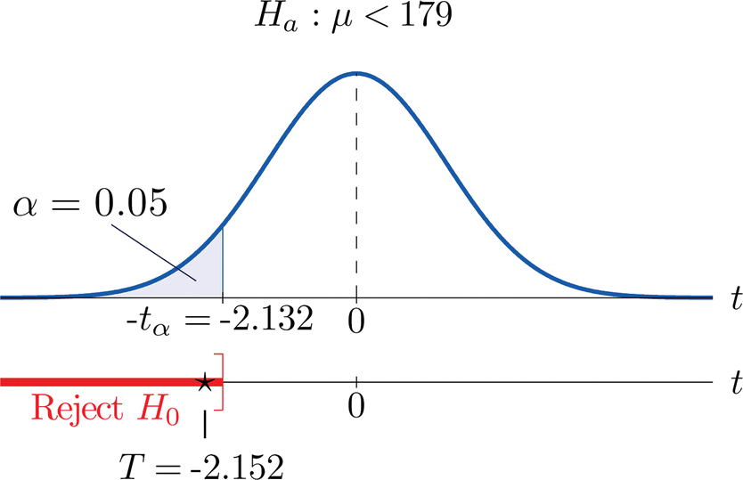
- Step 4. Since the symbol in \(H_a\) is “\(<\)” this is a left-tailed test, so there is a single critical value, \(-t_\alpha =-t_{0.05}[df=4]\). Reading from the row labeled \(df=4\) in Figure 7.1.6 its value is \(-2.132\). The rejection region is \((-\infty ,-2.132]\).
- Step 5. As shown in Figure \(\PageIndex{2}\) the test statistic falls in the rejection region. The decision is to reject \(H_0\). In the context of the problem our conclusion is:
The data provide sufficient evidence, at the \(5\%\) level of significance, to conclude that the average price of such rackets purchased at online auctions is less than \(\$179\).

To perform the test in Example \(\PageIndex{1}\) using the \(p\)-value approach, look in the row in Figure 7.1.6 with the heading \(df=4\) and search for the two \(t\)-values that bracket the unsigned value \(2.152\) of the test statistic. They are \(2.132\) and \(2.776\), in the columns with headings \(t_{0.050}\) and \(t_{0.025}\). They cut off right tails of area \(0.050\) and \(0.025\), so because \(2.152\) is between them it must cut off a tail of area between \(0.050\) and \(0.025\). By symmetry \(-2.152\) cuts off a left tail of area between \(0.050\) and \(0.025\), hence the \(p\)-value corresponding to \(t=-2.152\) is between \(0.025\) and \(0.05\). Although its precise value is unknown, it must be less than \(\alpha =0.05\), so the decision is to reject \(H_0\).
A small component in an electronic device has two small holes where another tiny part is fitted. In the manufacturing process the average distance between the two holes must be tightly controlled at \(0.02\) mm, else many units would be defective and wasted. Many times throughout the day quality control engineers take a small sample of the components from the production line, measure the distance between the two holes, and make adjustments if needed. Suppose at one time four units are taken and the distances are measured as
Determine, at the \(1\%\) level of significance, if there is sufficient evidence in the sample to conclude that an adjustment is needed. Assume the distances of interest are normally distributed.
Solution
- Step 1. The assumption is that the process is under control unless there is strong evidence to the contrary. Since a deviation of the average distance to either side is undesirable, the relevant test is \[H_0: \mu =0.02\\ \text{vs}\\ H_a: \mu \neq 0.02\; @\; \alpha =0.01 \nonumber \] where \(\mu\) denotes the mean distance between the holes.
- Step 2. The sample is small and the population standard deviation is unknown. Thus the test statistic is \[T=\frac{\bar{x}-\mu _0}{s /\sqrt{n}} \nonumber \] and has the Student \(t\)-distribution with \(n-1=4-1=3\) degrees of freedom.
- Step 3. From the data we compute \(\bar{x}=0.02075\) and \(s=0.00171\). Inserting these values into the formula for the test statistic gives \[T=\frac{\bar{x}-\mu _0}{s /\sqrt{n}}=\frac{0.02075-0.02}{0.00171\sqrt{4}}=0.877 \nonumber \]
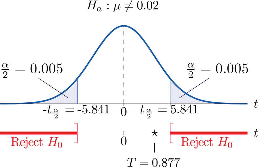
- Step 4. Since the symbol in \(H_a\) is “\(\neq\)” this is a two-tailed test, so there are two critical values, \(\pm t_{\alpha/2} =-t_{0.005}[df=3]\). Reading from the row in Figure 7.1.6 labeled \(df=3\) their values are \(\pm 5.841\). The rejection region is \((-\infty ,-5.841]\cup [5.841,\infty )\).
- Step 5. As shown in Figure \(\PageIndex{3}\) the test statistic does not fall in the rejection region. The decision is not to reject \(H_0\). In the context of the problem our conclusion is:
The data do not provide sufficient evidence, at the \(1\%\) level of significance, to conclude that the mean distance between the holes in the component differs from \(0.02\) mm.

To perform the test in "Example \(\PageIndex{2}\)" using the \(p\)-value approach, look in the row in Figure 7.1.6 with the heading \(df=3\) and search for the two \(t\)-values that bracket the value \(0.877\) of the test statistic. Actually \(0.877\) is smaller than the smallest number in the row, which is \(0.978\), in the column with heading \(t_{0.200}\). The value \(0.978\) cuts off a right tail of area \(0.200\), so because \(0.877\) is to its left it must cut off a tail of area greater than \(0.200\). Thus the \(p\)-value, which is the double of the area cut off (since the test is two-tailed), is greater than \(0.400\). Although its precise value is unknown, it must be greater than \(\alpha =0.01\), so the decision is not to reject \(H_0\).
Key Takeaway
- There are two formulas for the test statistic in testing hypotheses about a population mean with small samples. One test statistic follows the standard normal distribution, the other Student’s \(t\)-distribution.
- The population standard deviation is used if it is known, otherwise the sample standard deviation is used.
- Either five-step procedure, critical value or \(p\)-value approach, is used with either test statistic.


