5.4: Areas of Tails of Distributions

Learning Objectives

• To learn how to find, for a normal random variable \(X\) and an area \(a\), the value \(x^\ast\) of \(X\) so that \(P(X<x^\ast )=a\) or that \(P(X>x^\ast )=a\), whichever is required.

Definition: Left and Right Tails

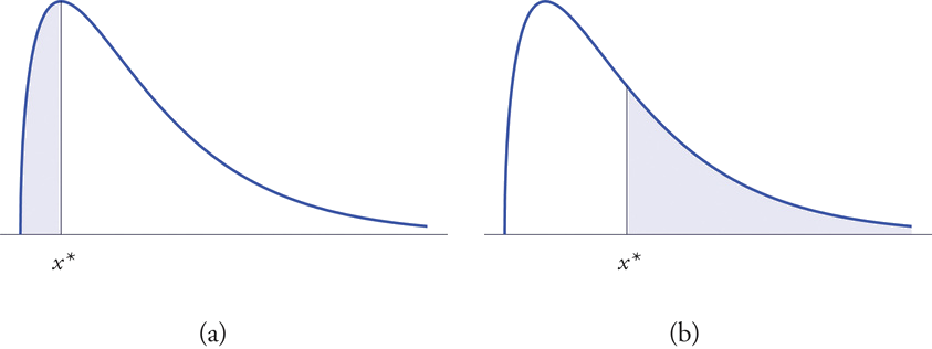
The left tail of a density curve \(y=f(x)\) of a continuous random variable \(X\) cut off by a value \(x^\ast\) of \(X\) is the region under the curve that is to the left of \(x^\ast\), as shown by the shading in Figure \(\PageIndex{1}\)(a). The right tail cut off by \(x^\ast\) is defined similarly, as indicated by the shading in Figure \(\PageIndex{1}\)(b).

Figure \(\PageIndex{1}\): Right and Left Tails of a Distribution

The probabilities tabulated in Figure 5.3.1 are areas of left tails in the standard normal distribution.

Tails of the Standard Normal Distribution

At times it is important to be able to solve the kind of problem illustrated by Figure \(\PageIndex{2}\). We have a certain specific area in mind, in this case the area \(0.0125\) of the shaded region in the figure, and we want to find the value \(z^\ast\) of \(Z\) that produces it. This is exactly the reverse of the kind of problems encountered so far. Instead of knowing a value \(z^\ast\) of \(Z\) and finding a corresponding area, we know the area and want to find \(z^\ast\). In the case at hand, in the terminology of the definition just above, we wish to find the value \(z^\ast\) that cuts off a left tail of area \(0.0125\) in the standard normal distribution.

The idea for solving such a problem is fairly simple, although sometimes its implementation can be a bit complicated. In a nutshell, one reads the cumulative probability table for \(Z\) in reverse, looking up the relevant area in the interior of the table and reading off the value of \(Z\) from the margins.

Figure \(\PageIndex{2}\): \(Z\) Value that Produces a Known Area

Example \(\PageIndex{1}\)

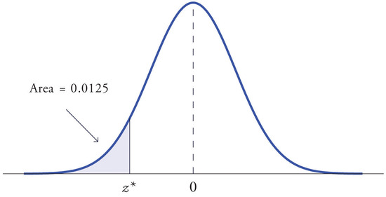
Find the value \(z^\ast\) of \(Z\) as determined by Figure \(\PageIndex{2}\): the value \(z^\ast\) that cuts off a left tail of area \(0.0125\) in the standard normal distribution. In symbols, find the number \(z^\ast\) such that \(P(Z<z^\ast )=0.0125\).

Solution

The number that is known, \(0.0125\), is the area of a left tail, and as already mentioned the probabilities tabulated in Figure 5.3.1 are areas of left tails. Thus to solve this problem we need only search in the interior of Figure 5.3.1 for the number \(0.0125\). It lies in the row with the heading \(-2.2\) and in the column with the heading \(0.04\). This means that \(P(Z < -2.24)= 0.0125\), hence \(z^\ast=-2.24\).

Example \(\PageIndex{2}\)

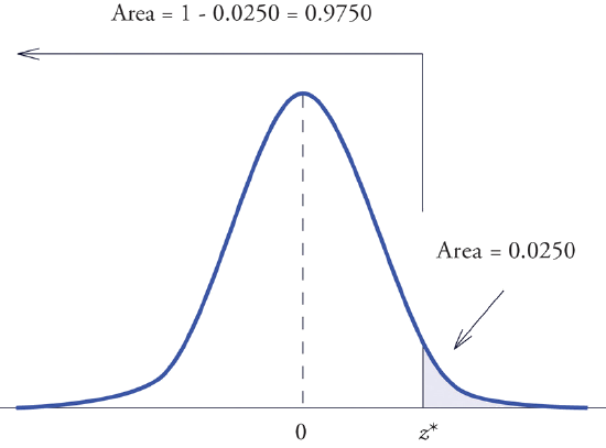
Find the value \(z^\ast\) of \(Z\) as determined by Figure \(\PageIndex{3}\): the value \(z^\ast\) that cuts off a right tail of area \(0.0250\) in the standard normal distribution. In symbols, find the number \(z^\ast\) such that \(P(Z >z^\ast)= 0.0250\).

Figure \(\PageIndex{3}\): \(Z\)Value that Produces a Known Area

Solution

The important distinction between this example and the previous one is that here it is the area of a right tail that is known. In order to be able to use Figure 5.3.1 we must first find that area of the left tail cut off by the unknown number \(z^\ast\). Since the total area under the density curve is \(1\), that area is \(1-0.0250=0.9750\). This is the number we look for in the interior of Figure 5.3.1. It lies in the row with the heading \(1.9\) and in the column with the heading \(0.06\). Therefore \(z^\ast=1.96\).

Definition: standard normal random variable

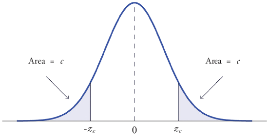
The value of the standard normal random variable \(Z\) that cuts off a right tail of area \(c\) is denoted \(z_c\). By symmetry, value of \(Z\) that cuts off a left tail of area \(c\) is \(-z_c\). See Figure \(\PageIndex{4}\).

Figure \(\PageIndex{4}\): The Numbers \(z_c\) and \(-z_c\)

The previous two examples were atypical because the areas we were looking for in the interior of Figure 5.3.1 were actually there. The following example illustrates the situation that is more common.

Example \(\PageIndex{3}\)

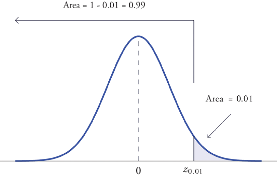
Find \(z_{.01}\) and \(-z_{.01}\), the values of \(Z\) that cut off right and left tails of area \(0.01\) in the standard normal distribution.

Solution

Since \(-z_{.01}\) cuts off a left tail of area \(0.01\) and Figure 5.3.1 is a table of left tails, we look for the number \(0.0100\) in the interior of the table. It is not there, but falls between the two numbers \(0.0102\) and \(0.0099\) in the row with heading \(-2.3\). The number \(0.0099\) is closer to \(0.0100\) than \(0.0102\) is, so for the hundredths place in \(-z_{.01}\) we use the heading of the column that contains \(0.0099\), namely, \(0.03\), and write \(-z_{.01}\approx -2.33\).

The answer to the second half of the problem is automatic: since \(-z_{.01}=-2.33\), we conclude immediately that \(z_{.01}=2.33\).

We could just as well have solved this problem by looking for \(z_{.01}\) first, and it is instructive to rework the problem this way. To begin with, we must first subtract \(0.01\) from \(1\) to find the area \(1-0.0100=0.9900\) of the left tail cut off by the unknown number \(z_{.01}\). See Figure \(\PageIndex{5}\). Then we search for the area \(0.9900\) in Figure \(\PageIndex{5}\). It is not there, but falls between the numbers \(0.9898\) and \(0.9901\) in the row with heading \(2.3\). Since \(0.9901\) is closer to \(0.9900\) than \(0.9898\) is, we use the column heading above it, \(0.03\), to obtain the approximation \(z_{.01}\approx 2.33\). Then finally \(-z_{.01}\approx -2.33\).

Figure \(\PageIndex{5}\): Computation of the Number \(z_{.01}\)

Tails of General Normal Distributions

The problem of finding the value \(x^\ast\) of a general normally distributed random variable \(X\) that cuts off a tail of a specified area also arises. This problem may be solved in two steps.

1. Suppose \(X\) is a normally distributed random variable with mean \(\mu\) and standard deviation \(\sigma\). To find the value \(x^\ast\) of \(X\) that cuts off a left or right tail of area \(c\) in the distribution of \(X\):
2. find the value \(z^\ast\) of \(Z\) that cuts off a left or right tail of area \(c\) in the standard normal distribution; \(z^\ast\) is the \(z\)-score of \(x^\ast\); compute \(x^\ast\) using the destandardization formula \[x^\ast =\mu +z^\ast \sigma \nonumber \]

In short, solve the corresponding problem for the standard normal distribution, thereby obtaining the \(z\)-score of \(x^\ast\), then destandardize to obtain \(x^\ast\).

Example \(\PageIndex{4}\)

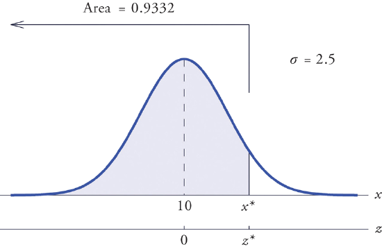
Find \(x^\ast\) such that \(P(X<x^\ast )=0.9332\), where \(X\) is a normal random variable with mean \(\mu =10\) and standard deviation \(\sigma =2.5\).

Solution

All the ideas for the solution are illustrated in Figure \(\PageIndex{6}\). Since \(0.9332\) is the area of a left tail, we can find \(z^\ast\) simply by looking for \(0.9332\) in the interior of Figure 5.3.1. It is in the row and column with headings \(1.5\) and \(0.00\), hence \(z^\ast=1.50\). Thus \(x^\ast\) is \(1.50\) standard deviations above the mean, so

\[x^\ast =\mu +z^\ast \sigma =10+(1.50)\cdot (0.2)=13.75 \nonumber \]

Figure \(\PageIndex{6}\): Tail of a Normally Distributed Random Variable

Example \(\PageIndex{5}\)

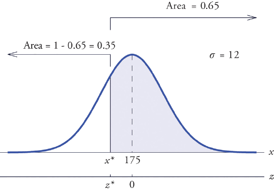
Find \(x^\ast\) such that \(P(X>x^\ast )=0.65\), where \(X\) is a normal random variable with mean \(\mu =175\) and standard deviation \(\sigma =12\).

Solution

The situation is illustrated in Figure \(\PageIndex{7}\). Since \(0.65\) is the area of a right tail, we first subtract it from \(1\) to obtain \(1-0.65=0.35\), the area of the complementary left tail. We find \(z^\ast\) by looking for \(0.3500\) in the interior of Figure 5.3.1. It is not present, but lies between table entries \(0.3520\) and \(0.3483\). The entry \(0.3483\) with row and column headings \(-0.3\) and \(0.09\) is closer to \(0.3500\) than the other entry is, so \(z^\ast \approx -0.39\). Thus \(x^\ast\) is \(0.39\) standard deviations below the mean, so

\[x^\ast =\mu +z^\ast \sigma =175+(-0.39)\cdot (12)=170.32 \nonumber \]

Figure \(\PageIndex{7}\): Tail of a Normally Distributed Random Variable

Example \(\PageIndex{6}\)

Scores on a standardized college entrance examination (CEE) are normally distributed with mean \(510\) and standard deviation \(60\). A selective university decides to give serious consideration for admission to applicants whose CEE scores are in the top \(5\%\) of all CEE scores. Find the minimum score that meets this criterion for serious consideration for admission.

Solution

Let \(X\) denote the score made on the CEE by a randomly selected individual. Then \(X\) is normally distributed with mean \(510\) and standard deviation \(60\). The probability that \(X\) lie in a particular interval is the same as the proportion of all exam scores that lie in that interval. Thus the minimum score that is in the top \(5\%\) of all CEE is the score \(x^\ast\) that cuts off a right tail in the distribution of \(X\) of area \(0.05\) (\(5\%\) expressed as a proportion). See Figure \(\PageIndex{8}\).

Figure \(\PageIndex{8}\): Tail of a Normally Distributed Random Variable

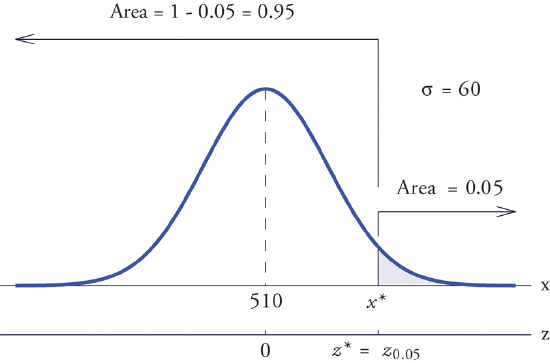
Since \(0.0500\) is the area of a right tail, we first subtract it from \(1\) to obtain \(1-0.0500=0.9500\), the area of the complementary left tail. We find \(z^\ast =z_{.05}\)by looking for \(0.9500\) in the interior of Figure 5.3.1. It is not present, and lies exactly half-way between the two nearest entries that are, \(0.9495\) and \(0.9505\). In the case of a tie like this, we will always average the values of \(Z\) corresponding to the two table entries, obtaining here the value \(z^\ast =1.645\). Using this value, we conclude that \(x^\ast\) is \(1.645\) standard deviations above the mean, so

\[x^\ast =\mu +z^\ast \sigma =510+(1.645)\cdot (60)=608.7 \nonumber \]

Example \(\PageIndex{7}\)

All boys at a military school must run a fixed course as fast as they can as part of a physical examination. Finishing times are normally distributed with mean \(29\) minutes and standard deviation \(2\) minutes. The middle \(75\%\) of all finishing times are classified as “average.” Find the range of times that are average finishing times by this definition.

Solution

Let \(X\) denote the finish time of a randomly selected boy. Then \(X\) is normally distributed with mean \(29\) and standard deviation \(2\). The probability that \(X\) lie in a particular interval is the same as the proportion of all finish times that lie in that interval. Thus the situation is as shown in Figure \(\PageIndex{9}\). Because the area in the middle corresponding to “average” times is \(0.75\), the areas of the two tails add up to \(1 - 0.75 = 0.25\) in all. By the symmetry of the density curve each tail must have half of this total, or area \(0.125\) each. Thus the fastest time that is “average” has \(z\)-score \(-z_{.125}\), which by Figure 5.3.1 is \(-1.15\), and the slowest time that is “average” has \(z\)-score \(z_{.125}=1.15\). The fastest and slowest times that are still considered average are

\[x_{fast}=\mu +(-z_{.125})\sigma =29+(-1.15)\cdot (2)=26.7 \nonumber \]

and

\[x_{slow}=\mu +z_{.125}\sigma =29+(1.15)\cdot (2)=31.3 \nonumber \]

Figure \(\PageIndex{9}\): Distribution of Times to Run a Course

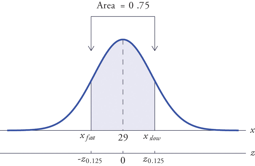
A boy has an average finishing time if he runs the course with a time between \(26.7\) and \(31.3\) minutes, or equivalently between \(26\) minutes \(42\) seconds and \(31\) minutes \(18\) seconds.

Key Takeaways

• The problem of finding the number \(z^\ast\) so that the probability \(P(Z<z^\ast )\) is a specified value \(c\) is solved by looking for the number \(c\) in the interior of Figure 5.3.1 and reading \(z^\ast\) from the margins.
• The problem of finding the number \(z^\ast\) so that the probability \(P(Z>z^\ast )\) is a specified value \(c\) is solved by looking for the complementary probability \(1-c\) in the interior of Figure 5.3.1 and reading \(z^\ast\) from the margins.
• For a normal random variable \(X\) with mean \(\mu\) and standard deviation \(\sigma\), the problem of finding the number \(x^\ast\) so that \(P(X<x^\ast )\) is a specified value \(c\) (or so that \(P(X>x^\ast )\) is a specified value \(c\)) is solved in two steps:
  • (1) solve the corresponding problem for \(Z\) with the same value of \(c\), thereby obtaining the \(z\)-score, \(z^\ast\), of \(x^\ast\);
  • (2) find \(x^\ast\) using \(x^\ast =\mu +z^\ast \sigma\).
• The value of \(Z\) that cuts off a right tail of area \(c\) in the standard normal distribution is denoted \(z_c\).