
4.2: Probability Distributions for Discrete Random Variables
- Page ID
- 561
\( \newcommand{\vecs}[1]{\overset { \scriptstyle \rightharpoonup} {\mathbf{#1}} } \)
\( \newcommand{\vecd}[1]{\overset{-\!-\!\rightharpoonup}{\vphantom{a}\smash {#1}}} \)
\( \newcommand{\dsum}{\displaystyle\sum\limits} \)
\( \newcommand{\dint}{\displaystyle\int\limits} \)
\( \newcommand{\dlim}{\displaystyle\lim\limits} \)
\( \newcommand{\id}{\mathrm{id}}\) \( \newcommand{\Span}{\mathrm{span}}\)
( \newcommand{\kernel}{\mathrm{null}\,}\) \( \newcommand{\range}{\mathrm{range}\,}\)
\( \newcommand{\RealPart}{\mathrm{Re}}\) \( \newcommand{\ImaginaryPart}{\mathrm{Im}}\)
\( \newcommand{\Argument}{\mathrm{Arg}}\) \( \newcommand{\norm}[1]{\| #1 \|}\)
\( \newcommand{\inner}[2]{\langle #1, #2 \rangle}\)
\( \newcommand{\Span}{\mathrm{span}}\)
\( \newcommand{\id}{\mathrm{id}}\)
\( \newcommand{\Span}{\mathrm{span}}\)
\( \newcommand{\kernel}{\mathrm{null}\,}\)
\( \newcommand{\range}{\mathrm{range}\,}\)
\( \newcommand{\RealPart}{\mathrm{Re}}\)
\( \newcommand{\ImaginaryPart}{\mathrm{Im}}\)
\( \newcommand{\Argument}{\mathrm{Arg}}\)
\( \newcommand{\norm}[1]{\| #1 \|}\)
\( \newcommand{\inner}[2]{\langle #1, #2 \rangle}\)
\( \newcommand{\Span}{\mathrm{span}}\) \( \newcommand{\AA}{\unicode[.8,0]{x212B}}\)
\( \newcommand{\vectorA}[1]{\vec{#1}} % arrow\)
\( \newcommand{\vectorAt}[1]{\vec{\text{#1}}} % arrow\)
\( \newcommand{\vectorB}[1]{\overset { \scriptstyle \rightharpoonup} {\mathbf{#1}} } \)
\( \newcommand{\vectorC}[1]{\textbf{#1}} \)
\( \newcommand{\vectorD}[1]{\overrightarrow{#1}} \)
\( \newcommand{\vectorDt}[1]{\overrightarrow{\text{#1}}} \)
\( \newcommand{\vectE}[1]{\overset{-\!-\!\rightharpoonup}{\vphantom{a}\smash{\mathbf {#1}}}} \)
\( \newcommand{\vecs}[1]{\overset { \scriptstyle \rightharpoonup} {\mathbf{#1}} } \)
\(\newcommand{\longvect}{\overrightarrow}\)
\( \newcommand{\vecd}[1]{\overset{-\!-\!\rightharpoonup}{\vphantom{a}\smash {#1}}} \)
\(\newcommand{\avec}{\mathbf a}\) \(\newcommand{\bvec}{\mathbf b}\) \(\newcommand{\cvec}{\mathbf c}\) \(\newcommand{\dvec}{\mathbf d}\) \(\newcommand{\dtil}{\widetilde{\mathbf d}}\) \(\newcommand{\evec}{\mathbf e}\) \(\newcommand{\fvec}{\mathbf f}\) \(\newcommand{\nvec}{\mathbf n}\) \(\newcommand{\pvec}{\mathbf p}\) \(\newcommand{\qvec}{\mathbf q}\) \(\newcommand{\svec}{\mathbf s}\) \(\newcommand{\tvec}{\mathbf t}\) \(\newcommand{\uvec}{\mathbf u}\) \(\newcommand{\vvec}{\mathbf v}\) \(\newcommand{\wvec}{\mathbf w}\) \(\newcommand{\xvec}{\mathbf x}\) \(\newcommand{\yvec}{\mathbf y}\) \(\newcommand{\zvec}{\mathbf z}\) \(\newcommand{\rvec}{\mathbf r}\) \(\newcommand{\mvec}{\mathbf m}\) \(\newcommand{\zerovec}{\mathbf 0}\) \(\newcommand{\onevec}{\mathbf 1}\) \(\newcommand{\real}{\mathbb R}\) \(\newcommand{\twovec}[2]{\left[\begin{array}{r}#1 \\ #2 \end{array}\right]}\) \(\newcommand{\ctwovec}[2]{\left[\begin{array}{c}#1 \\ #2 \end{array}\right]}\) \(\newcommand{\threevec}[3]{\left[\begin{array}{r}#1 \\ #2 \\ #3 \end{array}\right]}\) \(\newcommand{\cthreevec}[3]{\left[\begin{array}{c}#1 \\ #2 \\ #3 \end{array}\right]}\) \(\newcommand{\fourvec}[4]{\left[\begin{array}{r}#1 \\ #2 \\ #3 \\ #4 \end{array}\right]}\) \(\newcommand{\cfourvec}[4]{\left[\begin{array}{c}#1 \\ #2 \\ #3 \\ #4 \end{array}\right]}\) \(\newcommand{\fivevec}[5]{\left[\begin{array}{r}#1 \\ #2 \\ #3 \\ #4 \\ #5 \\ \end{array}\right]}\) \(\newcommand{\cfivevec}[5]{\left[\begin{array}{c}#1 \\ #2 \\ #3 \\ #4 \\ #5 \\ \end{array}\right]}\) \(\newcommand{\mattwo}[4]{\left[\begin{array}{rr}#1 \amp #2 \\ #3 \amp #4 \\ \end{array}\right]}\) \(\newcommand{\laspan}[1]{\text{Span}\{#1\}}\) \(\newcommand{\bcal}{\cal B}\) \(\newcommand{\ccal}{\cal C}\) \(\newcommand{\scal}{\cal S}\) \(\newcommand{\wcal}{\cal W}\) \(\newcommand{\ecal}{\cal E}\) \(\newcommand{\coords}[2]{\left\{#1\right\}_{#2}}\) \(\newcommand{\gray}[1]{\color{gray}{#1}}\) \(\newcommand{\lgray}[1]{\color{lightgray}{#1}}\) \(\newcommand{\rank}{\operatorname{rank}}\) \(\newcommand{\row}{\text{Row}}\) \(\newcommand{\col}{\text{Col}}\) \(\renewcommand{\row}{\text{Row}}\) \(\newcommand{\nul}{\text{Nul}}\) \(\newcommand{\var}{\text{Var}}\) \(\newcommand{\corr}{\text{corr}}\) \(\newcommand{\len}[1]{\left|#1\right|}\) \(\newcommand{\bbar}{\overline{\bvec}}\) \(\newcommand{\bhat}{\widehat{\bvec}}\) \(\newcommand{\bperp}{\bvec^\perp}\) \(\newcommand{\xhat}{\widehat{\xvec}}\) \(\newcommand{\vhat}{\widehat{\vvec}}\) \(\newcommand{\uhat}{\widehat{\uvec}}\) \(\newcommand{\what}{\widehat{\wvec}}\) \(\newcommand{\Sighat}{\widehat{\Sigma}}\) \(\newcommand{\lt}{<}\) \(\newcommand{\gt}{>}\) \(\newcommand{\amp}{&}\) \(\definecolor{fillinmathshade}{gray}{0.9}\)
- To learn the concept of the probability distribution of a discrete random variable.
- To learn the concepts of the mean, variance, and standard deviation of a discrete random variable, and how to compute them.
Associated to each possible value \(x\) of a discrete random variable \(X\) is the probability \(P(x)\) that \(X\) will take the value \(x\) in one trial of the experiment.
The probability distribution of a discrete random variable \(X\) is a list of each possible value of \(X\) together with the probability that \(X\) takes that value in one trial of the experiment.
The probabilities in the probability distribution of a random variable \(X\) must satisfy the following two conditions:
- Each probability \(P(x)\) must be between \(0\) and \(1\): \[0\leq P(x)\leq 1. \nonumber \]
- The sum of all the possible probabilities is \(1\): \[\sum P(x)=1. \nonumber \]
A fair coin is tossed twice. Let \(X\) be the number of heads that are observed.
- Construct the probability distribution of \(X\).
- Find the probability that at least one head is observed.
Solution
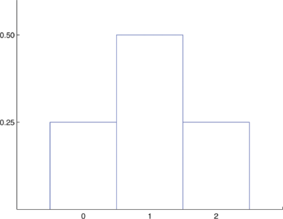
- The possible values that \(X\) can take are \(0\), \(1\), and \(2\). Each of these numbers corresponds to an event in the sample space \(S=\{hh,ht,th,tt\}\) of equally likely outcomes for this experiment: \[X = 0\; \text{to}\; \{tt\},\; X = 1\; \text{to}\; \{ht,th\}, \; \text{and}\; X = 2\; \text{to}\; {hh}. \nonumber \] The probability of each of these events, hence of the corresponding value of \(X\), can be found simply by counting, to give \[\begin{array}{c|ccc} x & 0 & 1 & 2 \\ \hline P(x) & 0.25 & 0.50 & 0.25\\ \end{array} \nonumber \] This table is the probability distribution of \(X\).
- “At least one head” is the event \(X\geq 1\), which is the union of the mutually exclusive events \(X = 1\) and \(X = 2\). Thus \[ \begin{align*} P(X\geq 1)&=P(1)+P(2)=0.50+0.25 \\[5pt] &=0.75 \end{align*} \nonumber \] A histogram that graphically illustrates the probability distribution is given in Figure \(\PageIndex{1}\).
A pair of fair dice is rolled. Let \(X\) denote the sum of the number of dots on the top faces.
- Construct the probability distribution of \(X\) for a paid of fair dice.
- Find \(P(X\geq 9)\).
- Find the probability that \(X\) takes an even value.
Solution
The sample space of equally likely outcomes is
\[\begin{matrix} 11 & 12 & 13 & 14 & 15 & 16\\ 21 & 22 & 23 & 24 & 25 & 26\\ 31 & 32 & 33 & 34 & 35 & 36\\ 41 & 42 & 43 & 44 & 45 & 46\\ 51 & 52 & 53 & 54 & 55 & 56\\ 61 & 62 & 63 & 64 & 65 & 66 \end{matrix} \nonumber \]
where the first digit is die 1 and the second number is die 2.
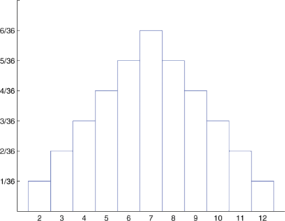
- The possible values for \(X\) are the numbers \(2\) through \(12\). \(X= 2\) is the event \(\{11\}\), so \(P(2)=1/36\). \(X= 3\) is the event \(\{12,21\}\), so \(P(3)=2/36\). Continuing this way we obtain the following table \[\begin{array}{c|ccccccccccc} x &2 &3 &4 &5 &6 &7 &8 &9 &10 &11 &12 \\ \hline P(x) &\dfrac{1}{36} &\dfrac{2}{36} &\dfrac{3}{36} &\dfrac{4}{36} &\dfrac{5}{36} &\dfrac{6}{36} &\dfrac{5}{36} &\dfrac{4}{36} &\dfrac{3}{36} &\dfrac{2}{36} &\dfrac{1}{36} \\ \end{array} \nonumber \]This table is the probability distribution of \(X\).
- The event \(X\geq 9\) is the union of the mutually exclusive events \(X = 9\), \(X = 10\), \(X = 11\), and \(X = 12\). Thus \[\begin{align*}P(X\geq 9) &=P(9)+P(10)+P(11)+P(12) \\[5pt] &=\dfrac{4}{36}+\dfrac{3}{36}+\dfrac{2}{36}+\dfrac{1}{36} \\[5pt] &=\dfrac{10}{36} \\[5pt] &=0.2\bar{7} \end{align*} \nonumber \]
- Before we immediately jump to the conclusion that the probability that \(X\) takes an even value must be \(0.5\), note that \(X\) takes six different even values but only five different odd values. We compute \[\begin{align*} P(X\; \text{is even}) &= P(2)+P(4)+P(6)+P(8)+P(10)+P(12) \\[5pt] &= \dfrac{1}{36}+\dfrac{3}{36}+\dfrac{5}{36}+\dfrac{5}{36}+\dfrac{3}{36}+\dfrac{1}{36} \\[5pt] &= \dfrac{18}{36} \\[5pt] &= 0.5 \end{align*} \nonumber \]A histogram that graphically illustrates the probability distribution is given in Figure \(\PageIndex{2}\).
The Mean and Standard Deviation of a Discrete Random Variable
The mean (also called the "expectation value" or "expected value") of a discrete random variable \(X\) is the number
\[\mu =E(X)=\sum x P(x) \label{mean} \]
The mean of a random variable may be interpreted as the average of the values assumed by the random variable in repeated trials of the experiment.
Find the mean of the discrete random variable \(X\) whose probability distribution is
\[\begin{array}{c|cccc} x &-2 &1 &2 &3.5\\ \hline P(x) &0.21 &0.34 &0.24 &0.21\\ \end{array} \nonumber \]
Solution
Using the definition of mean (Equation \ref{mean}) gives
\[\begin{align*} \mu &= \sum x P(x)\\[5pt] &= (-2)(0.21)+(1)(0.34)+(2)(0.24)+(3.5)(0.21)\\[5pt] &= 1.135 \end{align*} \nonumber \]
A service organization in a large town organizes a raffle each month. One thousand raffle tickets are sold for \(\$1\) each. Each has an equal chance of winning. First prize is \(\$300\), second prize is \(\$200\), and third prize is \(\$100\). Let \(X\) denote the net gain from the purchase of one ticket.
- Construct the probability distribution of \(X\).
- Find the probability of winning any money in the purchase of one ticket.
- Find the expected value of \(X\), and interpret its meaning.
Solution
- If a ticket is selected as the first prize winner, the net gain to the purchaser is the \(\$300\) prize less the \(\$1\) that was paid for the ticket, hence \(X = 300-11 = 299\). There is one such ticket, so \(P(299) = 0.001\). Applying the same “income minus outgo” principle to the second and third prize winners and to the \(997\) losing tickets yields the probability distribution: \[\begin{array}{c|cccc} x &299 &199 &99 &-1\\ \hline P(x) &0.001 &0.001 &0.001 &0.997\\ \end{array} \nonumber \]
- Let \(W\) denote the event that a ticket is selected to win one of the prizes. Using the table \[\begin{align*} P(W)&=P(299)+P(199)+P(99)=0.001+0.001+0.001\\[5pt] &=0.003 \end{align*} \nonumber \]
- Using the definition of expected value (Equation \ref{mean}), \[\begin{align*}E(X)&=(299)\cdot (0.001)+(199)\cdot (0.001)+(99)\cdot (0.001)+(-1)\cdot (0.997) \\[5pt] &=-0.4 \end{align*} \nonumber \] The negative value means that one loses money on the average. In particular, if someone were to buy tickets repeatedly, then although he would win now and then, on average he would lose \(40\) cents per ticket purchased.
The concept of expected value is also basic to the insurance industry, as the following simplified example illustrates.
A life insurance company will sell a \(\$200,000\) one-year term life insurance policy to an individual in a particular risk group for a premium of \(\$195\). Find the expected value to the company of a single policy if a person in this risk group has a \(99.97\%\) chance of surviving one year.
Solution
Let \(X\) denote the net gain to the company from the sale of one such policy. There are two possibilities: the insured person lives the whole year or the insured person dies before the year is up. Applying the “income minus outgo” principle, in the former case the value of \(X\) is \(195-0\); in the latter case it is \(195-200,000=-199,805\). Since the probability in the first case is 0.9997 and in the second case is \(1-0.9997=0.0003\), the probability distribution for \(X\) is:
\[\begin{array}{c|cc} x &195 &-199,805 \\ \hline P(x) &0.9997 &0.0003 \\ \end{array}\nonumber \]
Therefore
\[\begin{align*} E(X) &=\sum x P(x) \\[5pt]&=(195)\cdot (0.9997)+(-199,805)\cdot (0.0003) \\[5pt] &=135 \end{align*} \nonumber \]
Occasionally (in fact, \(3\) times in \(10,000\)) the company loses a large amount of money on a policy, but typically it gains \(\$195\), which by our computation of \(E(X)\) works out to a net gain of \(\$135\) per policy sold, on average.
The variance (\(\sigma ^2\)) of a discrete random variable \(X\) is the number
\[\sigma ^2=\sum (x-\mu )^2P(x) \label{var1} \]
which by algebra is equivalent to the formula
\[\sigma ^2=\left [ \sum x^2 P(x)\right ]-\mu ^2 \label{var2} \]
The standard deviation, \(\sigma \), of a discrete random variable \(X\) is the square root of its variance, hence is given by the formulas
\[\sigma =\sqrt{\sum (x-\mu )^2P(x)}=\sqrt{\left [ \sum x^2 P(x)\right ]-\mu ^2} \label{std} \]
The variance and standard deviation of a discrete random variable \(X\) may be interpreted as measures of the variability of the values assumed by the random variable in repeated trials of the experiment. The units on the standard deviation match those of \(X\).
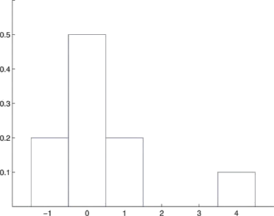
A discrete random variable \(X\) has the following probability distribution:
\[\begin{array}{c|cccc} x &-1 &0 &1 &4\\ \hline P(x) &0.2 &0.5 &a &0.1\\ \end{array} \label{Ex61} \]
A histogram that graphically illustrates the probability distribution is given in Figure \(\PageIndex{3}\).
Compute each of the following quantities.
- \(a\).
- \(P(0)\).
- \(P(X> 0)\).
- \(P(X\geq 0)\).
- \(P(X\leq -2)\).
- The mean \(\mu \) of \(X\).
- The variance \(\sigma ^2\) of \(X\).
- The standard deviation \(\sigma \) of \(X\).
Solution
- Since all probabilities must add up to 1, \[a=1-(0.2+0.5+0.1)=0.2 \nonumber \]
- Directly from the table, P(0)=0.5\[P(0)=0.5 \nonumber \]
- From Table \ref{Ex61}, \[P(X> 0)=P(1)+P(4)=0.2+0.1=0.3 \nonumber \]
- From Table \ref{Ex61}, \[P(X\geq 0)=P(0)+P(1)+P(4)=0.5+0.2+0.1=0.8 \nonumber \]
- Since none of the numbers listed as possible values for \(X\) is less than or equal to \(-2\), the event \(X\leq -2\) is impossible, so \[P(X\leq -2)=0 \nonumber \]
- Using the formula in the definition of \(\mu \) (Equation \ref{mean}) \[\begin{align*}\mu &=\sum x P(x) \\[5pt] &=(-1)\cdot (0.2)+(0)\cdot (0.5)+(1)\cdot (0.2)+(4)\cdot (0.1) \\[5pt] &=0.4 \end{align*} \nonumber \]
- Using the formula in the definition of \(\sigma ^2\) (Equation \ref{var1}) and the value of \(\mu \) that was just computed, \[\begin{align*} \sigma ^2 &=\sum (x-\mu )^2P(x) \\ &= (-1-0.4)^2\cdot (0.2)+(0-0.4)^2\cdot (0.5)+(1-0.4)^2\cdot (0.2)+(4-0.4)^2\cdot (0.1)\\ &= 1.84 \end{align*} \nonumber \]
- Using the result of part (g), \(\sigma =\sqrt{1.84}=1.3565\)
Summary
- The probability distribution of a discrete random variable \(X\) is a listing of each possible value \(x\) taken by \(X\) along with the probability \(P(x)\) that \(X\) takes that value in one trial of the experiment.
- The mean \(\mu \) of a discrete random variable \(X\) is a number that indicates the average value of \(X\) over numerous trials of the experiment. It is computed using the formula \(\mu =\sum xP(x)\).
- The variance \(\sigma ^2\) and standard deviation \(\sigma \) of a discrete random variable \(X\) are numbers that indicate the variability of \(X\) over numerous trials of the experiment. They may be computed using the formula \(\sigma ^2=\left [ \sum x^2P(x) \right ]-\mu ^2\).