
3.3: Conditional Probability and Independent Events
- Page ID
- 532
\( \newcommand{\vecs}[1]{\overset { \scriptstyle \rightharpoonup} {\mathbf{#1}} } \)
\( \newcommand{\vecd}[1]{\overset{-\!-\!\rightharpoonup}{\vphantom{a}\smash {#1}}} \)
\( \newcommand{\id}{\mathrm{id}}\) \( \newcommand{\Span}{\mathrm{span}}\)
( \newcommand{\kernel}{\mathrm{null}\,}\) \( \newcommand{\range}{\mathrm{range}\,}\)
\( \newcommand{\RealPart}{\mathrm{Re}}\) \( \newcommand{\ImaginaryPart}{\mathrm{Im}}\)
\( \newcommand{\Argument}{\mathrm{Arg}}\) \( \newcommand{\norm}[1]{\| #1 \|}\)
\( \newcommand{\inner}[2]{\langle #1, #2 \rangle}\)
\( \newcommand{\Span}{\mathrm{span}}\)
\( \newcommand{\id}{\mathrm{id}}\)
\( \newcommand{\Span}{\mathrm{span}}\)
\( \newcommand{\kernel}{\mathrm{null}\,}\)
\( \newcommand{\range}{\mathrm{range}\,}\)
\( \newcommand{\RealPart}{\mathrm{Re}}\)
\( \newcommand{\ImaginaryPart}{\mathrm{Im}}\)
\( \newcommand{\Argument}{\mathrm{Arg}}\)
\( \newcommand{\norm}[1]{\| #1 \|}\)
\( \newcommand{\inner}[2]{\langle #1, #2 \rangle}\)
\( \newcommand{\Span}{\mathrm{span}}\) \( \newcommand{\AA}{\unicode[.8,0]{x212B}}\)
\( \newcommand{\vectorA}[1]{\vec{#1}} % arrow\)
\( \newcommand{\vectorAt}[1]{\vec{\text{#1}}} % arrow\)
\( \newcommand{\vectorB}[1]{\overset { \scriptstyle \rightharpoonup} {\mathbf{#1}} } \)
\( \newcommand{\vectorC}[1]{\textbf{#1}} \)
\( \newcommand{\vectorD}[1]{\overrightarrow{#1}} \)
\( \newcommand{\vectorDt}[1]{\overrightarrow{\text{#1}}} \)
\( \newcommand{\vectE}[1]{\overset{-\!-\!\rightharpoonup}{\vphantom{a}\smash{\mathbf {#1}}}} \)
\( \newcommand{\vecs}[1]{\overset { \scriptstyle \rightharpoonup} {\mathbf{#1}} } \)
\( \newcommand{\vecd}[1]{\overset{-\!-\!\rightharpoonup}{\vphantom{a}\smash {#1}}} \)
\(\newcommand{\avec}{\mathbf a}\) \(\newcommand{\bvec}{\mathbf b}\) \(\newcommand{\cvec}{\mathbf c}\) \(\newcommand{\dvec}{\mathbf d}\) \(\newcommand{\dtil}{\widetilde{\mathbf d}}\) \(\newcommand{\evec}{\mathbf e}\) \(\newcommand{\fvec}{\mathbf f}\) \(\newcommand{\nvec}{\mathbf n}\) \(\newcommand{\pvec}{\mathbf p}\) \(\newcommand{\qvec}{\mathbf q}\) \(\newcommand{\svec}{\mathbf s}\) \(\newcommand{\tvec}{\mathbf t}\) \(\newcommand{\uvec}{\mathbf u}\) \(\newcommand{\vvec}{\mathbf v}\) \(\newcommand{\wvec}{\mathbf w}\) \(\newcommand{\xvec}{\mathbf x}\) \(\newcommand{\yvec}{\mathbf y}\) \(\newcommand{\zvec}{\mathbf z}\) \(\newcommand{\rvec}{\mathbf r}\) \(\newcommand{\mvec}{\mathbf m}\) \(\newcommand{\zerovec}{\mathbf 0}\) \(\newcommand{\onevec}{\mathbf 1}\) \(\newcommand{\real}{\mathbb R}\) \(\newcommand{\twovec}[2]{\left[\begin{array}{r}#1 \\ #2 \end{array}\right]}\) \(\newcommand{\ctwovec}[2]{\left[\begin{array}{c}#1 \\ #2 \end{array}\right]}\) \(\newcommand{\threevec}[3]{\left[\begin{array}{r}#1 \\ #2 \\ #3 \end{array}\right]}\) \(\newcommand{\cthreevec}[3]{\left[\begin{array}{c}#1 \\ #2 \\ #3 \end{array}\right]}\) \(\newcommand{\fourvec}[4]{\left[\begin{array}{r}#1 \\ #2 \\ #3 \\ #4 \end{array}\right]}\) \(\newcommand{\cfourvec}[4]{\left[\begin{array}{c}#1 \\ #2 \\ #3 \\ #4 \end{array}\right]}\) \(\newcommand{\fivevec}[5]{\left[\begin{array}{r}#1 \\ #2 \\ #3 \\ #4 \\ #5 \\ \end{array}\right]}\) \(\newcommand{\cfivevec}[5]{\left[\begin{array}{c}#1 \\ #2 \\ #3 \\ #4 \\ #5 \\ \end{array}\right]}\) \(\newcommand{\mattwo}[4]{\left[\begin{array}{rr}#1 \amp #2 \\ #3 \amp #4 \\ \end{array}\right]}\) \(\newcommand{\laspan}[1]{\text{Span}\{#1\}}\) \(\newcommand{\bcal}{\cal B}\) \(\newcommand{\ccal}{\cal C}\) \(\newcommand{\scal}{\cal S}\) \(\newcommand{\wcal}{\cal W}\) \(\newcommand{\ecal}{\cal E}\) \(\newcommand{\coords}[2]{\left\{#1\right\}_{#2}}\) \(\newcommand{\gray}[1]{\color{gray}{#1}}\) \(\newcommand{\lgray}[1]{\color{lightgray}{#1}}\) \(\newcommand{\rank}{\operatorname{rank}}\) \(\newcommand{\row}{\text{Row}}\) \(\newcommand{\col}{\text{Col}}\) \(\renewcommand{\row}{\text{Row}}\) \(\newcommand{\nul}{\text{Nul}}\) \(\newcommand{\var}{\text{Var}}\) \(\newcommand{\corr}{\text{corr}}\) \(\newcommand{\len}[1]{\left|#1\right|}\) \(\newcommand{\bbar}{\overline{\bvec}}\) \(\newcommand{\bhat}{\widehat{\bvec}}\) \(\newcommand{\bperp}{\bvec^\perp}\) \(\newcommand{\xhat}{\widehat{\xvec}}\) \(\newcommand{\vhat}{\widehat{\vvec}}\) \(\newcommand{\uhat}{\widehat{\uvec}}\) \(\newcommand{\what}{\widehat{\wvec}}\) \(\newcommand{\Sighat}{\widehat{\Sigma}}\) \(\newcommand{\lt}{<}\) \(\newcommand{\gt}{>}\) \(\newcommand{\amp}{&}\) \(\definecolor{fillinmathshade}{gray}{0.9}\)- To learn the concept of a conditional probability and how to compute it.
- To learn the concept of independence of events, and how to apply it.
Suppose a fair die has been rolled and you are asked to give the probability that it was a five. There are six equally likely outcomes, so your answer is \(1/6\). But suppose that before you give your answer you are given the extra information that the number rolled was odd. Since there are only three odd numbers that are possible, one of which is five, you would certai: nly revise your estimate of the likelihood that a five was rolled from \(1/6\) to \(1/3\). In general, the revised probability that an event A has occurred, taking into account the additional information that another event \(B\) has definitely occurred on this trial of the experiment, is called the conditional probability of \(A\) given \(B\) and is denoted by \(P(A\mid B)\). The reasoning employed in this example can be generalized to yield the computational formula in the following definition.
The conditional probability of \(A\) given \(B\), denoted \(P(A\mid B)\), is the probability that event \(A\) has occurred in a trial of a random experiment for which it is known that event \(B\) has definitely occurred. It may be computed by means of the following formula:
\[P(A\mid B)=\dfrac{P(A\cap B)}{P(B)} \label{CondProb} \]
A fair (unbiased) die is rolled.
- Find the probability that the number rolled is a five, given that it is odd.
- Find the probability that the number rolled is odd, given that it is a five.
Solution
The sample space for this experiment is the set \(S={1,2,3,4,5,6}\) consisting of six equally likely outcomes. Let \(F\) denote the event “a five is rolled” and let \(O\) denote the event “an odd number is rolled,” so that
\[F={5}\; \; \text{and}\; \; O={1,3,5} \nonumber \]
- This is the introductory example, so we already know that the answer is \(1/3\). To use Equation \ref{CondProb} to confirm this we must replace \(A\) in the formula (the event whose likelihood we seek to estimate) by \(F\) and replace \(B\) (the event we know for certain has occurred) by \(O\): \[P(F\mid O)=\dfrac{P(F\cap O)}{P(O)}\nonumber \] Since \[F\cap O={5}\cap {1,3,5}={5},\; P(F\cap O)=1/6 \nonumber \]Since \[O={1,3,5}, \; P(O)=3/6. \nonumber \]Thus \[P(F\mid O)=\dfrac{P(F\cap O)}{P(O)}=\dfrac{1/6}{3/6}=\dfrac{1}{3} \nonumber \]
- This is the same problem, but with the roles of \(F\) and \(O\) reversed. Since we are given that the number that was rolled is five, which is odd, the probability in question must be \(1\). To apply Equation \ref{CondProb} to this case we must now replace \(A\) (the event whose likelihood we seek to estimate) by \(O\) and \(B\) (the event we know for certain has occurred) by \(F\):\[P(O\mid F)=\dfrac{P(O\cap F)}{P(F)} \nonumber \]Obviously \(P(F)=1/6\). In part (a) we found that \(P(F\mid O)=1/6\). Thus\[P(O\mid F)=\dfrac{P(O\cap F)}{P(F)}=\dfrac{1/6}{1/6}=1 \nonumber \]
Just as we did not need the computational formula in this example, we do not need it when the information is presented in a two-way classification table, as in the next example.
In a sample of \(902\) individuals under \(40\) who were or had previously been married, each person was classified according to gender and age at first marriage. The results are summarized in the following two-way classification table, where the meaning of the labels is:
- \(M\): male
- \(F\): female
- \(E\): a teenager when first married
- \(W\): in one’s twenties when first married
- \(H\): in one’s thirties when first married
| \(E\) | \(W\) | \(H\) | Total | |
|---|---|---|---|---|
| \(M\) | 43 | 293 | 114 | 450 |
| \(F\) | 82 | 299 | 71 | 452 |
| Total | 125 | 592 | 185 | 902 |
The numbers in the first row mean that \(43\) people in the sample were men who were first married in their teens, \(293\) were men who were first married in their twenties, \(114\) men who were first married in their thirties, and a total of \(450\) people in the sample were men. Similarly for the numbers in the second row. The numbers in the last row mean that, irrespective of gender, \(125\) people in the sample were married in their teens, \(592\) in their twenties, \(185\) in their thirties, and that there were \(902\) people in the sample in all. Suppose that the proportions in the sample accurately reflect those in the population of all individuals in the population who are under \(40\) and who are or have previously been married. Suppose such a person is selected at random.
- Find the probability that the individual selected was a teenager at first marriage.
- Find the probability that the individual selected was a teenager at first marriage, given that the person is male.
Solution
It is natural to let \(E\) also denote the event that the person selected was a teenager at first marriage and to let \(M\) denote the event that the person selected is male.
- According to the table, the proportion of individuals in the sample who were in their teens at their first marriage is \(125/902\). This is the relative frequency of such people in the population, hence \(P(E)=125/902\approx 0.139\) or about \(14\%\).
- Since it is known that the person selected is male, all the females may be removed from consideration, so that only the row in the table corresponding to men in the sample applies:
| \(E\) | \(W\) | \(H\) | Total | |
|---|---|---|---|---|
| \(M\) | 43 | 293 | 114 | 450 |
The proportion of males in the sample who were in their teens at their first marriage is \(43/450\). This is the relative frequency of such people in the population of males, hence \(P(E/M)=43/450\approx 0.096\) or about \(10\%\).
In the next example, the computational formula in the definition must be used.
Suppose that in an adult population the proportion of people who are both overweight and suffer hypertension is \(0.09\); the proportion of people who are not overweight but suffer hypertension is \(0.11\); the proportion of people who are overweight but do not suffer hypertension is \(0.02\); and the proportion of people who are neither overweight nor suffer hypertension is \(0.78\). An adult is randomly selected from this population.
- Find the probability that the person selected suffers hypertension given that he is overweight.
- Find the probability that the selected person suffers hypertension given that he is not overweight.
- Compare the two probabilities just found to give an answer to the question as to whether overweight people tend to suffer from hypertension.
Let \(H\) denote the event “the person selected suffers hypertension.” Let \(O\) denote the event “the person selected is overweight.” The probability information given in the problem may be organized into the following contingency table:
| \(O\) | \(O^c\) | |
|---|---|---|
| \(H\) | 0.09 | 0.11 |
| \(H^c\) | 0.02 | 0.78 |
- Using the formula in the definition of conditional probability (Equation \ref{CondProb}), \[P(H|O)=\dfrac{P(H\cap O)}{P(O)}=\dfrac{0.09}{0.09+0.02}=0.8182 \nonumber \]
- Using the formula in the definition of conditional probability (Equation \ref{CondProb}), \[P(H|O)=\dfrac{P(H\cap O^c)}{P(O^c)}=\dfrac{0.11}{0.11+0.78}=0.1236 \nonumber \]
- \(P(H|O)=0.8182\) is over six times as large as \(P(H|O^c)=0.1236\), which indicates a much higher rate of hypertension among people who are overweight than among people who are not overweight. It might be interesting to note that a direct comparison of \(P(H\cap O)=0.09\) and \(P(H\cap O^c)=0.11\) does not answer the same question.
Independent Events
Although typically we expect the conditional probability \(P(A\mid B)\) to be different from the probability \(P(A)\) of \(A\), it does not have to be different from \(P(A)\). When \(P(A\mid B)=P(A)\), the occurrence of \(B\) has no effect on the likelihood of \(A\). Whether or not the event \(A\) has occurred is independent of the event \(B\).
Using algebra it can be shown that the equality \(P(A\mid B)=P(A)\) holds if and only if the equality \(P(A\cap B)=P(A)\cdot P(B)\) holds, which in turn is true if and only if \(P(B\mid A)=P(B)\). This is the basis for the following definition.
Events \(A\) and \(B\) are independent (i.e., events whose probability of occurring together is the product of their individual probabilities). if
\[P(A\cap B)=P(A)\cdot P(B) \nonumber \]
If \(A\) and \(B\) are not independent then they are dependent.
The formula in the definition has two practical but exactly opposite uses:
- In a situation in which we can compute all three probabilities \(P(A), P(B)\; \text{and}\; P(A\cap B)\), it is used to check whether or not the events \(A\) and \(B\) are independent:
- If \(P(A\cap B)=P(A)\cdot P(B)\), then \(A\) and \(B\) are independent.
- If \(P(A\cap B)\neq P(A)\cdot P(B)\), then \(A\) and \(B\) are not independent.
- In a situation in which each of \(P(A)\) and \(P(B)\) can be computed and it is known that \(A\) and \(B\) are independent, then we can compute \(P(A\cap B)\) by multiplying together \(P(A) \; \text{and}\; P(B)\): \(P(A\cap B)=P(A)\cdot P(B)\).
A single fair die is rolled. Let \(A=\{3\}\) and \(B=\{1,3,5\}\). Are \(A\) and \(B\) independent?
Solution
In this example we can compute all three probabilities \(P(A)=1/6\), \(P(B)=1/2\), and \(P(A\cap B)=P(\{3\})=1/6\). Since the product \(P(A)\cdot P(B)=(1/6)(1/2)=1/12\) is not the same number as \(P(A\cap B)=1/6\), the events \(A\) and \(B\) are not independent.
The two-way classification of married or previously married adults under \(40\) according to gender and age at first marriage produced the table
| E | W | H | Total | |
|---|---|---|---|---|
| M | 43 | 293 | 114 | 450 |
| F | 82 | 299 | 71 | 452 |
| Total | 125 | 592 | 185 | 902 |
Determine whether or not the events \(F\): “female” and \(E\): “was a teenager at first marriage” are independent.
Solution
The table shows that in the sample of \(902\) such adults, \(452\) were female, \(125\) were teenagers at their first marriage, and \(82\) were females who were teenagers at their first marriage, so that
\[ \begin{align*} P(F) &=\dfrac{452}{902},\\[4pt] P(E) &=\dfrac{125}{902} \\[4pt] P(F\cap E) &=\dfrac{82}{902} \end{align*} \nonumber \]
Since
\[ \begin{align*} P(F)\cdot P(E) &=\dfrac{452}{902}\cdot \dfrac{125}{902} \\[4pt] &=0.069 \end{align*} \nonumber \]
is not the same as
\[P(F\cap E)=\dfrac{82}{902}=0.091 \nonumber \]
we conclude that the two events are not independent.
Many diagnostic tests for detecting diseases do not test for the disease directly but for a chemical or biological product of the disease, hence are not perfectly reliable. The sensitivity of a test is the probability that the test will be positive when administered to a person who has the disease. The higher the sensitivity, the greater the detection rate and the lower the false negative rate.
Suppose the sensitivity of a diagnostic procedure to test whether a person has a particular disease is \(92\%\). A person who actually has the disease is tested for it using this procedure by two independent laboratories.
- What is the probability that both test results will be positive?
- What is the probability that at least one of the two test results will be positive?
Solution
- Let \(A_1\) denote the event “the test by the first laboratory is positive” and let \(A_2\) denote the event “the test by the second laboratory is positive.” Since \(A_1\) and \(A_2\) are independent, \[\begin{align*} P(A_1\cap A_2) &=P(A_1)\cdot P(A_2) \\[4pt] &=0.92\times 0.92 \\[4pt] &=0.8464 \end{align*} \nonumber \]
- Using the Additive Rule for Probability and the probability just computed, \[\begin{align*}P(A_1\cup A_2) &= P(A_1)+P(A_2)-P(A_1\cap A_2) \\[4pt] &=0.92+0.92-0.8464 \\[4pt] &=0.9936 \end{align*} \nonumber \]
The specificity of a diagnostic test for a disease is the probability that the test will be negative when administered to a person who does not have the disease. The higher the specificity, the lower the false positive rate. Suppose the specificity of a diagnostic procedure to test whether a person has a particular disease is \(89\%\).
- A person who does not have the disease is tested for it using this procedure. What is the probability that the test result will be positive?
- A person who does not have the disease is tested for it by two independent laboratories using this procedure. What is the probability that both test results will be positive?
Solution
- Let \(B\) denote the event “the test result is positive.” The complement of \(B\) is that the test result is negative, and has probability the specificity of the test, \(0.89\). Thus \[P(B)=1-P(B^c)=1-0.89=0.11 \nonumber \]
- Let \(B_1\) denote the event “the test by the first laboratory is positive” and let \(B_2\) denote the event “the test by the second laboratory is positive.” Since \(B_1\) and \(B_2\) are independent, by part (a) of the example \[P(B_1\cap B_2)=P(B_1)\cdot P(B_2)=0.11\times 0.11=0.0121 \nonumber \]
The concept of independence applies to any number of events. For example, three events \(A,\; B,\; \text{and}\; C\) are independent if \(P(A\cap B\cap C)=P(A)\cdot P(B)\cdot P(C)\). Note carefully that, as is the case with just two events, this is not a formula that is always valid, but holds precisely when the events in question are independent.
The reliability of a system can be enhanced by redundancy, which means building two or more independent devices to do the same job, such as two independent braking systems in an automobile. Suppose a particular species of trained dogs has a \(90\%\) chance of detecting contraband in airline luggage. If the luggage is checked three times by three different dogs independently of one another, what is the probability that contraband will be detected?
Solution
Let \(D_1\) denote the event that the contraband is detected by the first dog, \(D_2\) the event that it is detected by the second dog, and \(D_3\) the event that it is detected by the third. Since each dog has a \(90\%\) of detecting the contraband, by the Probability Rule for Complements it has a \(10\%\) chance of failing. In symbols, \[P(D_{1}^{c})=0.10,\; \; P(D_{2}^{c})=0.10,\; \; P(D_{3}^{c})=0.10 \nonumber \]
Let \(D\) denote the event that the contraband is detected. We seek \(P(D)\). It is easier to find \(P(D^c)\), because although there are several ways for the contraband to be detected, there is only one way for it to go undetected: all three dogs must fail. Thus \(D^c=D_{1}^{c}\cap D_{2}^{c}\cap D_{3}^{c}\) and \[P(D)=1-P(D^c)=1-P(D_{1}^{c}\cap D_{2}^{c}\cap D_{3}^{c}) \nonumber \]But the events \(D_1\), \(D_2\), and \(D_3\) are independent, which implies that their complements are independent, so \[P(D_{1}^{c}\cap D_{2}^{c}\cap D_{3}^{c})=P(D_{1}^{c})\cdot P(D_{2}^{c})\cdot P(D_{3}^{c})=0.10\times 0.10\times 0.10=0.001 \nonumber \]
Using this number in the previous display we obtain \[P(D)=1-0.001=0.999 \nonumber \]
That is, although any one dog has only a \(90\%\) chance of detecting the contraband, three dogs working independently have a \(99.9\%\) chance of detecting it.
Probabilities on Tree Diagrams
Some probability problems are made much simpler when approached using a tree diagram. The next example illustrates how to place probabilities on a tree diagram and use it to solve a problem.
A jar contains \(10\) marbles, \(7\) black and \(3\) white. Two marbles are drawn without replacement, which means that the first one is not put back before the second one is drawn.
- What is the probability that both marbles are black?
- What is the probability that exactly one marble is black?
- What is the probability that at least one marble is black?
Solution
A tree diagram for the situation of drawing one marble after the other without replacement is shown in Figure \(\PageIndex{1}\). The circle and rectangle will be explained later, and should be ignored for now.
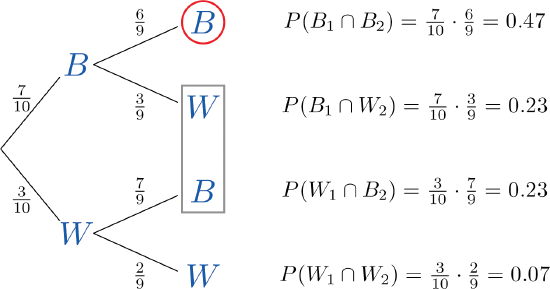
The numbers on the two leftmost branches are the probabilities of getting either a black marble, \(7\) out of \(10\), or a white marble, \(3\) out of \(10\), on the first draw. The number on each remaining branch is the probability of the event corresponding to the node on the right end of the branch occurring, given that the event corresponding to the node on the left end of the branch has occurred. Thus for the top branch, connecting the two Bs, it is \(P(B_2\mid B_1)\), where \(B_1\) denotes the event “the first marble drawn is black” and \(B_2\) denotes the event “the second marble drawn is black.” Since after drawing a black marble out there are \(9\) marbles left, of which \(6\) are black, this probability is \(6/9\).
The number to the right of each final node is computed as shown, using the principle that if the formula in the Conditional Rule for Probability is multiplied by \(P(B)\), then the result is
\[P(B\cap A)=P(B)\cdot P(A\mid B) \nonumber \]
- The event “both marbles are black” is \(B_1\cap B_2\) and corresponds to the top right node in the tree, which has been circled. Thus as indicated there, it is \(0.47\).
- The event “exactly one marble is black” corresponds to the two nodes of the tree enclosed by the rectangle. The events that correspond to these two nodes are mutually exclusive: black followed by white is incompatible with white followed by black. Thus in accordance with the Additive Rule for Probability we merely add the two probabilities next to these nodes, since what would be subtracted from the sum is zero. Thus the probability of drawing exactly one black marble in two tries is \(0.23+0.23=0.46\).
- The event “at least one marble is black” corresponds to the three nodes of the tree enclosed by either the circle or the rectangle. The events that correspond to these nodes are mutually exclusive, so as in part (b) we merely add the probabilities next to these nodes. Thus the probability of drawing at least one black marble in two tries is \(0.47+0.23+0.23=0.93\).
Of course, this answer could have been found more easily using the Probability Law for Complements, simply subtracting the probability of the complementary event, “two white marbles are drawn,” from 1 to obtain \(1-0.07=0.93\).
As this example shows, finding the probability for each branch is fairly straightforward, since we compute it knowing everything that has happened in the sequence of steps so far. Two principles that are true in general emerge from this example:
- The probability of the event corresponding to any node on a tree is the product of the numbers on the unique path of branches that leads to that node from the start.
- If an event corresponds to several final nodes, then its probability is obtained by adding the numbers next to those nodes.
Key Takeaway
- A conditional probability is the probability that an event has occurred, taking into account additional information about the result of the experiment.
- A conditional probability can always be computed using the formula in the definition. Sometimes it can be computed by discarding part of the sample space.
- Two events \(A\) and \(B\) are independent if the probability \(P(A\cap B)\) of their intersection \(A\cap B\) is equal to the product \(P(A)\cdot P(B)\) of their individual probabilities.