21.1: Analysis Lab
- Page ID
- 2236
\( \newcommand{\vecs}[1]{\overset { \scriptstyle \rightharpoonup} {\mathbf{#1}} } \)
\( \newcommand{\vecd}[1]{\overset{-\!-\!\rightharpoonup}{\vphantom{a}\smash {#1}}} \)
\( \newcommand{\dsum}{\displaystyle\sum\limits} \)
\( \newcommand{\dint}{\displaystyle\int\limits} \)
\( \newcommand{\dlim}{\displaystyle\lim\limits} \)
\( \newcommand{\id}{\mathrm{id}}\) \( \newcommand{\Span}{\mathrm{span}}\)
( \newcommand{\kernel}{\mathrm{null}\,}\) \( \newcommand{\range}{\mathrm{range}\,}\)
\( \newcommand{\RealPart}{\mathrm{Re}}\) \( \newcommand{\ImaginaryPart}{\mathrm{Im}}\)
\( \newcommand{\Argument}{\mathrm{Arg}}\) \( \newcommand{\norm}[1]{\| #1 \|}\)
\( \newcommand{\inner}[2]{\langle #1, #2 \rangle}\)
\( \newcommand{\Span}{\mathrm{span}}\)
\( \newcommand{\id}{\mathrm{id}}\)
\( \newcommand{\Span}{\mathrm{span}}\)
\( \newcommand{\kernel}{\mathrm{null}\,}\)
\( \newcommand{\range}{\mathrm{range}\,}\)
\( \newcommand{\RealPart}{\mathrm{Re}}\)
\( \newcommand{\ImaginaryPart}{\mathrm{Im}}\)
\( \newcommand{\Argument}{\mathrm{Arg}}\)
\( \newcommand{\norm}[1]{\| #1 \|}\)
\( \newcommand{\inner}[2]{\langle #1, #2 \rangle}\)
\( \newcommand{\Span}{\mathrm{span}}\) \( \newcommand{\AA}{\unicode[.8,0]{x212B}}\)
\( \newcommand{\vectorA}[1]{\vec{#1}} % arrow\)
\( \newcommand{\vectorAt}[1]{\vec{\text{#1}}} % arrow\)
\( \newcommand{\vectorB}[1]{\overset { \scriptstyle \rightharpoonup} {\mathbf{#1}} } \)
\( \newcommand{\vectorC}[1]{\textbf{#1}} \)
\( \newcommand{\vectorD}[1]{\overrightarrow{#1}} \)
\( \newcommand{\vectorDt}[1]{\overrightarrow{\text{#1}}} \)
\( \newcommand{\vectE}[1]{\overset{-\!-\!\rightharpoonup}{\vphantom{a}\smash{\mathbf {#1}}}} \)
\( \newcommand{\vecs}[1]{\overset { \scriptstyle \rightharpoonup} {\mathbf{#1}} } \)
\(\newcommand{\longvect}{\overrightarrow}\)
\( \newcommand{\vecd}[1]{\overset{-\!-\!\rightharpoonup}{\vphantom{a}\smash {#1}}} \)
\(\newcommand{\avec}{\mathbf a}\) \(\newcommand{\bvec}{\mathbf b}\) \(\newcommand{\cvec}{\mathbf c}\) \(\newcommand{\dvec}{\mathbf d}\) \(\newcommand{\dtil}{\widetilde{\mathbf d}}\) \(\newcommand{\evec}{\mathbf e}\) \(\newcommand{\fvec}{\mathbf f}\) \(\newcommand{\nvec}{\mathbf n}\) \(\newcommand{\pvec}{\mathbf p}\) \(\newcommand{\qvec}{\mathbf q}\) \(\newcommand{\svec}{\mathbf s}\) \(\newcommand{\tvec}{\mathbf t}\) \(\newcommand{\uvec}{\mathbf u}\) \(\newcommand{\vvec}{\mathbf v}\) \(\newcommand{\wvec}{\mathbf w}\) \(\newcommand{\xvec}{\mathbf x}\) \(\newcommand{\yvec}{\mathbf y}\) \(\newcommand{\zvec}{\mathbf z}\) \(\newcommand{\rvec}{\mathbf r}\) \(\newcommand{\mvec}{\mathbf m}\) \(\newcommand{\zerovec}{\mathbf 0}\) \(\newcommand{\onevec}{\mathbf 1}\) \(\newcommand{\real}{\mathbb R}\) \(\newcommand{\twovec}[2]{\left[\begin{array}{r}#1 \\ #2 \end{array}\right]}\) \(\newcommand{\ctwovec}[2]{\left[\begin{array}{c}#1 \\ #2 \end{array}\right]}\) \(\newcommand{\threevec}[3]{\left[\begin{array}{r}#1 \\ #2 \\ #3 \end{array}\right]}\) \(\newcommand{\cthreevec}[3]{\left[\begin{array}{c}#1 \\ #2 \\ #3 \end{array}\right]}\) \(\newcommand{\fourvec}[4]{\left[\begin{array}{r}#1 \\ #2 \\ #3 \\ #4 \end{array}\right]}\) \(\newcommand{\cfourvec}[4]{\left[\begin{array}{c}#1 \\ #2 \\ #3 \\ #4 \end{array}\right]}\) \(\newcommand{\fivevec}[5]{\left[\begin{array}{r}#1 \\ #2 \\ #3 \\ #4 \\ #5 \\ \end{array}\right]}\) \(\newcommand{\cfivevec}[5]{\left[\begin{array}{c}#1 \\ #2 \\ #3 \\ #4 \\ #5 \\ \end{array}\right]}\) \(\newcommand{\mattwo}[4]{\left[\begin{array}{rr}#1 \amp #2 \\ #3 \amp #4 \\ \end{array}\right]}\) \(\newcommand{\laspan}[1]{\text{Span}\{#1\}}\) \(\newcommand{\bcal}{\cal B}\) \(\newcommand{\ccal}{\cal C}\) \(\newcommand{\scal}{\cal S}\) \(\newcommand{\wcal}{\cal W}\) \(\newcommand{\ecal}{\cal E}\) \(\newcommand{\coords}[2]{\left\{#1\right\}_{#2}}\) \(\newcommand{\gray}[1]{\color{gray}{#1}}\) \(\newcommand{\lgray}[1]{\color{lightgray}{#1}}\) \(\newcommand{\rank}{\operatorname{rank}}\) \(\newcommand{\row}{\text{Row}}\) \(\newcommand{\col}{\text{Col}}\) \(\renewcommand{\row}{\text{Row}}\) \(\newcommand{\nul}{\text{Nul}}\) \(\newcommand{\var}{\text{Var}}\) \(\newcommand{\corr}{\text{corr}}\) \(\newcommand{\len}[1]{\left|#1\right|}\) \(\newcommand{\bbar}{\overline{\bvec}}\) \(\newcommand{\bhat}{\widehat{\bvec}}\) \(\newcommand{\bperp}{\bvec^\perp}\) \(\newcommand{\xhat}{\widehat{\xvec}}\) \(\newcommand{\vhat}{\widehat{\vvec}}\) \(\newcommand{\uhat}{\widehat{\uvec}}\) \(\newcommand{\what}{\widehat{\wvec}}\) \(\newcommand{\Sighat}{\widehat{\Sigma}}\) \(\newcommand{\lt}{<}\) \(\newcommand{\gt}{>}\) \(\newcommand{\amp}{&}\) \(\definecolor{fillinmathshade}{gray}{0.9}\)Learning Objectives
- To study the Analysis Lab calculator
General Instructions
Analysis Lab that can perform basic descriptive and inferential statistics. Descriptive statistics include the graphic methods: box plots, histograms, stem and leaf displays, and normal quantile plots. Inferential statistics include independent-group t tests, Chi Square tests, tests in simple regression/correlation, and Analysis of Variance.
Reading/Entering Data
There are currently two "libraries" of datasets. The default library is "RVLS_data." You can change the library by using the pop-up menu. Just under the pop-up menu for libraries is a pop-up menu of datasets in the library. Choose the dataset you want to analyze. A description of the dataset will be shown on the right side of the display. The data from the case studies will be included in the near future.
To enter your own data, click the button labeled "Enter/Edit User Data." A window will open with an area for you to enter or paste in your data. You may get a warning that you must use the keyboard shortcut to paste because your system may not allow Java programs to read the clipboard. Pasting formatted text will not work. If you have trouble pasting in your data, try pasting them as unformatted text into Word, copying, and then pasting into Analysis Lab.
The first line should contain the names of the variables (separated by spaces or tabs). The remaining lines should contain the data themselves. Missing data cannot be handled so all observations must have valid data for all variables. All variables must be numeric. If one of your variables is to be used as a "Grouping" or "Classification" variable, then values of the grouping variable must be integers ranging from one to the total number of groups. Use grouping variables so that you can do a separate analysis for each level of the variable or to use the variable as an independent variable in an analysis of variance. Once you have entered your data, click on the "Accept data" button. The data will be temporarily saved so that if you click the "Enter/Edit User Data" button again they will be shown
Choosing Variables
To analyze a variable, select it in the "\(Y\)" pop-up menu and then click on the type of analysis you wish to perform. To see the relationship between two variables, select one in the "\(X\)" menu and the other in the "\(Y\)" menu. Then click on the "Correlation/regression" button. Specify a grouping variable to do an analysis separately for each group of observations. You also specify a grouping variable to conduct an analysis of variance or do a t test.
Copying/Printing
Analysis Lab does not have any copying or printing capabilities. However, you can copy and(optionally) print by doing a screen capture. If you are using a Macintosh with OSX, press "\(4\)" while holding down the command (Apple), shift, and control keys. You will be given the opportunity to select an area of the screen to be copied to the clipboard.
If you are using Windows, make sure the window you want to copy is selected. Then, hold down the ALT key and press the Print Screen Key key. The window will be copied to the clipboard for pasting into another application such as a word processor.
Problems
On occasion, some browsers do not refresh the display. If you get a blank window, try resizing it slightly.
ANOVA Instructions
The following information is a guide to doing Analysis of Variance (ANOVA) with Analysis Lab. Analysis Lab was designed to allow the most common types of designs to be analyzed with a minimum of effort.
One Between-Subjects Variable
This analysis is used when there are two or more independent groups of subjects and one score per subject.
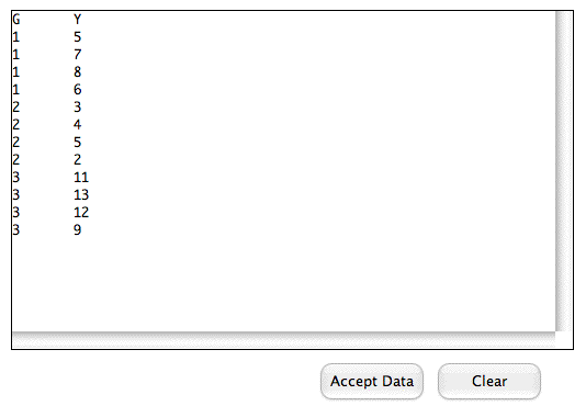
- The data should be arranged so that there is one variable that indicates group membership and a second variable that contains the dependent variable. The variable indicating group membership must use consecutive integers (e.g., \(1, 2, 3\)) as group indicators. The data below have two variables; \(G\) for group membership and \(Y\) for the dependent variable. There are three groups and four observations (subjects) per group.
| G | Y |
| 1 | 5 |
| 1 | 7 |
| 1 | 8 |
| 1 | 6 |
| 2 | 3 |
| 2 | 4 |
| 2 | 5 |
| 2 | 2 |
| 3 | 11 |
| 3 | 13 |
| 3 | 12 |
| 3 | 9 |
- Paste the data into analysis lab.
- Copy your data.
- Click the Enter/Edit data button.
- Paste the data using keyboard shortcuts (Control-V for Windows, CMD-V for Macs). Then click "Accept Data."
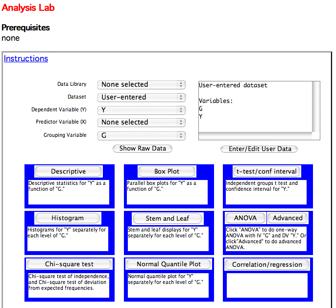
Choose \(Y\) as the dependent variable and \(G\) as the grouping variable as shown. Then click the ANOVA button. Note that the description says what analysis will be done. \(IV\) stands for "Independent Variable" and \(DV\) stands for "Dependent Variable."
- The ANOVA summary table will be presented.

One Within-Subjects Variable
Use this design when you have one group of observations (subjects) with two or more scores per observation.
- Format your data so that each row contains all the data for one observation. Each score is a separate variable. For the following example, there are five observations with three scores per observation. The variable names are \(T1\), \(T2\), and \(T3\).
| T1 | T2 | T3 |
| 2 | 3 | 4 |
| 3 | 5 | 4 |
| 2 | 4 | 6 |
| 1 | 3 | 3 |
| 6 | 7 | 9 |
- Paste the data into analysis lab (see the instructions for One-Way Between-Subjects).
- Click the "Advanced" button next to the ANOVA" button.
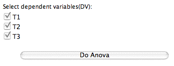
- Select the dependent variables you want to analyze. and click the "Do Anova" button. Here the variables \(T1\), and \(T2\), and \(T3\) are chosen.
- The Summary Table is presented. The effect \(DV\) stands for "Dependent Variable." It is a test of the within-subjects variable.

Two or More Between-Subject Variables
Use this design when you have more than one between-subject variable and only one score per subject. In the following example, the variables are \(A\) and \(B\). The variable \(A\) has two levels and the variable \(B\) has three levels. There are \(3\) scores per "cell." A cell is a combination of one level of \(A\) and one level of \(B\).
Note that Analysis Lab uses unweighted means analysis rather than the general linear model. This will give slightly different results from most other programs when there are unequal sample sizes and the degrees of freedom are greater than one.
- Format the data so that there is one variable indicating the level of each independent variable. The variable must use consecutive integer variables. There is also a dependent variable. In the example, the variable \(A\) indicates the level of the variable \(A\), \(B\) indicates the level of the variable \(B\), and \(Y\) is the dependent variable.
| A | B | Y |
| 1 | 1 | 3 |
| 1 | 1 | 5 |
| 1 | 1 | 4 |
| 1 | 2 | 7 |
| 1 | 2 | 6 |
| 1 | 2 | 8 |
| 1 | 3 | 4 |
| 1 | 3 | 9 |
| 1 | 3 | 6 |
| 2 | 1 | 9 |
| 2 | 1 | 9 |
| 2 | 1 | 10 |
| 2 | 2 | 13 |
| 2 | 2 | 11 |
| 2 | 2 | 14 |
| 2 | 3 | 6 |
| 2 | 3 | 7 |
| 2 | 3 | 9 |
- Paste the data into analysis lab (see the instructions for One-Way Between-Subjects).
- Click the "Advanced" button next to the ANOVA" button.
- Choose the dependent variable and the independent variables. The independent variables are called "group variables." Then click the "Do Anova" button.
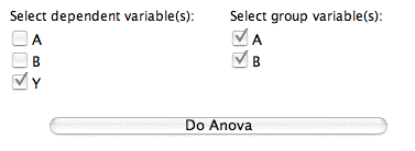
- The Summary table is shown below.

One or More Between-Subject Variables and one Within-Subject Variable
- Format the data so that a variable indicates each level of each between-subject variable. Include more than one dependent variable. For this example, there is one between-subjects variable (\(A\)) with two levels and one within-subjects variable (\(T\)) with four levels.
| A | T1 | T2 | T3 | T4 |
| 1 | 5 | 4 | 3 | 6 |
| 1 | 7 | 6 | 2 | 9 |
| 1 | 6 | 5 | 7 | 5 |
| 2 | 8 | 9 | 12 | 14 |
| 2 | 6 | 7 | 9 | 11 |
| 2 | 2 | 4 | 3 | 6 |
- Paste the data into analysis lab (see the instructions for One-Way Between-Subjects).
- Click the "Advanced" button next to the ANOVA" button.
- Choose the dependent variables and the independent variables. The independent variables are called "group variables." In this example there is one independent variable (\(A\)) and four dependent variables (\(T1\), \(T2\), \(T3\), and \(T4\)). Then click the "Do Anova" button.
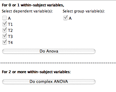
- The Summary table is shown. \(DV\) stands for dependent variable and is the effect of the within-subjects factor. \(A \times DV\) is the interaction of the between-subjects variable and the within-subjects variable.

One or More Between-Subjects Variables and Two more More Within-Subjects Variables
- Format the data so that a variable indicates each level of each between-subject variable. Include more than one dependent variable. For this example, there are two between-subjects variable (Age and Gender) and two within-subjects variable (Day and Trial ). There are four groups of subjects (the combination of two levels of Age and two levels of Gender). Each subject is given two trials a day for two days. For convenience \(A\) is used as an abbreviation for age, \(G\) for Gender, \(D\) for Day, and \(T\) for Trial. The variable \(D1T1\) is the score for \(\text{Day 1 Trial 1}\), \(D1T2\) for \(\text{Day 1, Trial 2}\), etc.
| A | B | D1T1 | D1T2 | D2T1 | D2T2 |
| 1 | 1 | 5 | 7 | 4 | 8 |
| 1 | 1 | 4 | 7 | 5 | 9 |
| 1 | 1 | 5 | 5 | 8 | 9 |
| 1 | 2 | 5 | 4 | 5 | 7 |
| 1 | 2 | 4 | 8 | 11 | 12 |
| 1 | 2 | 8 | 7 | 6 | 5 |
| 2 | 1 | 12 | 13 | 12 | 15 |
| 2 | 1 | 10 | 9 | 11 | 13 |
| 2 | 1 | 8 | 8 | 7 | 15 |
| 2 | 2 | 13 | 14 | 11 | 12 |
| 2 | 2 | 7 | 5 | 8 | 7 |
| 2 | 2 | 9 | 11 | 11 | 10 |
- Paste the data into analysis lab (see the instructions for One-Way Between-Subjects).
- Click the "Advanced" button next to the ANOVA" button.
- Choose the dependent variables and the independent variables. The independent variables are called "group variables." In this example there are two independent variable (\(A\) and \(B\)) and four dependent variables (\(D1T1\), \(D1T2\), \(D2T1\), and \(D2T2\)). Then click the "Do Complex Anova" at the bottom of the window.
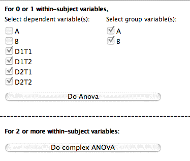
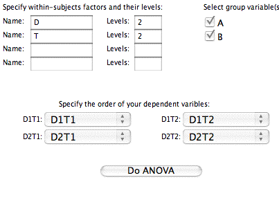
- Next you name the within-subject variables and specify the number of levels of each. Since there are two days and two trials per day, both of the values are two. Analysis Lab allows up to four. In this example there are two ( \(D\) and \(T\)). Also indicate that \(A\) and \(B\) are the between-subjects (group) variables.
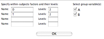
- Next you will be asked to associate the variable names to the levels of the variables. The way the variables were named in this example makes this a trivial exercise. However, if you used other variable names, it would take a little effort. Click the "Do ANOVA" button when finished.
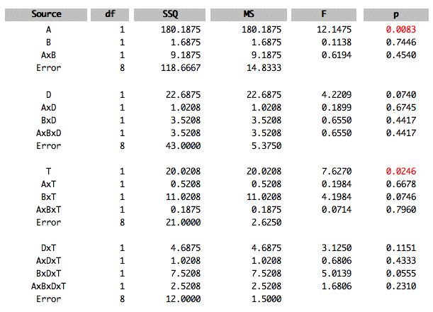
- The Summary Table is presented.
