12.7: Correlated Pairs
- Page ID
- 2342
Learning Objectives
- Determine whether you have correlated pairs or independent groups
- Compute a t test for correlated pairs
Let's consider how to analyze the data from the "ADHD Treatment" case study. These data consist of the scores of \(24\) children with ADHD on a delay of gratification (DOG) task. Each child was tested under four dosage levels. In this section, we will be concerned only with testing the difference between the mean of the placebo (\(D0\)) condition and the mean of the highest dosage condition (\(D60\)). The first question is why the difference between means should not be tested using the procedure described in the section Difference Between Two Means (Independent Groups). The answer lies in the fact that in this experiment we do not have independent groups. The scores in the \(D0\) condition are from the same subjects as the scores in the \(D60\) condition. There is only one group of subjects, each subject being tested in both the \(D0\) and \(D60\) conditions.
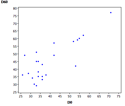
Figure \(\PageIndex{1}\) shows a scatter plot of the \(60\)-mg scores (\(D60\)) as a function of the \(0\)-mg scores (\(D0\)). It is clear that children who get more correct in the \(D0\) condition tend to get more correct in the \(D60\) condition. The correlation between the two conditions is high: \(r = 0.80\). Clearly these two variables are not independent.

Computations
You may recall that the method to test the difference between these means was presented in the section on "Testing a Single Mean." The computational procedure is to compute the difference between the \(D60\) and the \(D0\) conditions for each child and test whether the mean difference is significantly different from \(0\). The difference scores are shown in Table \(\PageIndex{1}\). As shown in the section on testing a single mean, the mean difference score is \(4.96\) which is significantly different from \(0\): \(t = 3.22,\; df = 23,\; p = 0.0038\). This \(t\) test has various names including "correlated \(t\) test" and "related-pairs \(t\) test".
In general, the correlated \(t\) test is computed by first computing the difference between the two scores for each subject. Then, a test of a single mean is computed on the mean of these difference scores.
| D0 | D60 | D60-D0 |
|---|---|---|
| 57 | 62 | 5 |
| 27 | 49 | 22 |
| 32 | 30 | -2 |
| 31 | 34 | 3 |
| 34 | 38 | 4 |
| 38 | 36 | -2 |
| 71 | 77 | 6 |
| 33 | 51 | 18 |
| 34 | 45 | 11 |
| 53 | 42 | -11 |
| 36 | 43 | 7 |
| 42 | 57 | 15 |
| 26 | 36 | 10 |
| 52 | 58 | 6 |
| 36 | 35 | -1 |
| 55 | 60 | 5 |
| 36 | 33 | -3 |
| 42 | 49 | 7 |
| 36 | 33 | -3 |
| 54 | 59 | 5 |
| 34 | 35 | 1 |
| 29 | 37 | 8 |
| 33 | 45 | 12 |
| 33 | 29 | -4 |
If you had mistakenly used the method for an independent-groups \(t\) test with these data, you would have found that \(t = 1.42\), \(df = 46\), and \(p = 0.15\). That is, the difference between means would not have been found to be statistically significant. This is a typical result: correlated \(t\) tests almost always have greater power than independent-groups \(t\) tests. This is because in correlated \(t\) tests, each difference score is a comparison of performance in one condition with the performance of that same subject in another condition. This makes each subject "their own control" and keeps differences between subjects from entering into the analysis. The result is that the standard error of the difference between means is smaller in the correlated \(t\) test and, since this term is in the denominator of the formula for \(t\), results in a larger \(t\).
Details about the Standard Error of the Difference between Means (Optional)
To see why the standard error of the difference between means is smaller in a correlated \(t\) test, consider the variance of difference scores. As shown in the section on the Variance Sum Law, the variance of the sum or difference of the two variables \(X\) and \(Y\) is:
\[S_{X\pm Y}^{2} = S_{X}^{2} + S_{Y}^{2} \pm 2rS_XS_Y\]
Therefore, the variance of difference scores is the variance in the first condition (\(X\)) plus the variance in the second condition (\(Y\)) minus twice the product of
- the correlation,
- the standard deviation of \(X\), and
- the standard deviation of \(Y\). For the current example, \(r = 0.80\) and the variances and standard deviations are shown in Table \(\PageIndex{2}\).
| D0 | D60 | D60 - D0 | |
|---|---|---|---|
| Variance | 128.02 | 151.78 | 56.82 |
| Sd | 11.31 | 12.32 | 7.54 |
The variance of the difference scores of \(56.82\) can be computed as:
\[128.02 + 151.78 - (2)(0.80)(11.31)(12.32)\]
which is equal to \(56.82\) except for rounding error. Notice that the higher the correlation, the lower the standard error of the mean.


