
15.3.6: Chapter 7 Lab
- Page ID
- 28620

\( \newcommand{\vecs}[1]{\overset { \scriptstyle \rightharpoonup} {\mathbf{#1}} } \) \( \newcommand{\vecd}[1]{\overset{-\!-\!\rightharpoonup}{\vphantom{a}\smash {#1}}} \)\(\newcommand{\id}{\mathrm{id}}\) \( \newcommand{\Span}{\mathrm{span}}\) \( \newcommand{\kernel}{\mathrm{null}\,}\) \( \newcommand{\range}{\mathrm{range}\,}\) \( \newcommand{\RealPart}{\mathrm{Re}}\) \( \newcommand{\ImaginaryPart}{\mathrm{Im}}\) \( \newcommand{\Argument}{\mathrm{Arg}}\) \( \newcommand{\norm}[1]{\| #1 \|}\) \( \newcommand{\inner}[2]{\langle #1, #2 \rangle}\) \( \newcommand{\Span}{\mathrm{span}}\) \(\newcommand{\id}{\mathrm{id}}\) \( \newcommand{\Span}{\mathrm{span}}\) \( \newcommand{\kernel}{\mathrm{null}\,}\) \( \newcommand{\range}{\mathrm{range}\,}\) \( \newcommand{\RealPart}{\mathrm{Re}}\) \( \newcommand{\ImaginaryPart}{\mathrm{Im}}\) \( \newcommand{\Argument}{\mathrm{Arg}}\) \( \newcommand{\norm}[1]{\| #1 \|}\) \( \newcommand{\inner}[2]{\langle #1, #2 \rangle}\) \( \newcommand{\Span}{\mathrm{span}}\)\(\newcommand{\AA}{\unicode[.8,0]{x212B}}\)
Modeling Continuous Random Variables
Open the Minitab file lab6.mpj from the website.
Simulate a Uniform Random Variable
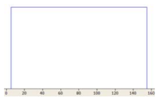
- The Uniform random variable is described by two parameters, the minimum and the maximum. Each value between the minimum and the maximum has the same probability of being chosen, so the uniform random variable has a rectangular shape. In this simulation, we will model the amount of concrete in a building supply store, which follows a uniform distribution from 20 to 180 tons.
- Using the formulas from the part 4 slides, find the population mean, median and standard deviation for this random variable.
- Use the column heading Uniform Sim to save data and simulate 1000 trials in Minitab (use the menu item CALC>RANDOM DATA and choose Uniform.) Use the command STAT>BASIC STATISTICS>GRAPHICAL SUMMARY to calculate the sample mean, sample median and sample standard deviation of the simulated data as well as a box plot and histogram, and paste the output here. Compare the sample statistics to the corresponding population values you calculated in part a.
- Describe the shape of the histogram. Does it appear to match the rectangular shape of the population probability graph shown above?
- Identify the minimum and maximum values. Are they near the values 20 and 180 that you used to define the model?
Simulate an Exponential Random Variable
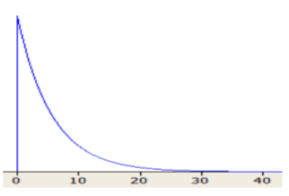
- The Exponential random variable is described by one parameter, the expected value or \(\mu\). The shape of the curve is an exponential decay model that we studied in Module 4. This random variable is often used to model the waiting time until an event occurs, in which the future waiting time is independent of the past waiting time. In this simulation, we will model trauma patients who arrive at a hospital’s Emergency Room at a rate of one every 7.2minutes (7.2 minutes is the expected value.).
- Using the formulas from the part 4 slides, find the population mean, median and standard deviation for this random variable.
- Use the column heading Exponential Sim to save data and simulate 1000 trials in Minitab (use the menu item CALC>RANDOM DATA and choose Exponential. The scale box will be \(\mu\) and the Threshold box should remain at 0.0 ) Use the command STAT>BASIC STATISTICS>GRAPHICAL SUMMARY to calculate the sample mean, sample median and sample standard deviation of the simulated data as well as a box plot and histogram, and paste the output here. Compare the sample statistics to the corresponding population values you calculated in part a.
- Describe the shape of the histogram. Does it appear to match the exponential decay shape of the population probability graph shown above?
- Identify the minimum and maximum values. Determine if the maximum value is an extreme outlier.
Simulate a Normal Random Variable
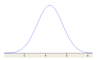
- The Normal random variable is described by two parameters, the expected value \(\mu\) and the population standard deviation \(\sigma\). The curve is bell‐shaped and frequently occurs in nature. In this simulation, we will model the popcorn cooking time, which follows a Normal random variable, with \(\mu=4.75\) minutes and \(\sigma=0.64\) minutes.
- Use the column heading Normal Sim to save data and simulate 1000 trials (use the menu item CALC>RANDOM DATA and choose Normal.) Use the command STAT>BASIC STATISTICS>GRAPHICAL SUMMARY to calculate the sample mean, sample median and sample standard deviation of the simulated data as well as a box plot and histogram, and paste the output here.
- Describe the shape of the histogram. Does it appear to match the bell‐shape of the population probability graph shown above?
- Identify the minimum and maximum values. Determine the \(Z\)‐score of each. Do these values seem to be extreme outliers?
- Compare the sample mean, median and standard deviation to the population values.