14.2: The Simple Linear Regression Model
- Page ID
- 20927

In the scatterplot example shown above, we saw linear correlation between the two dependent variables. We are now going to create a statistical model relating these two variables, but let’s start by reviewing a mathematical linear model from algebra:
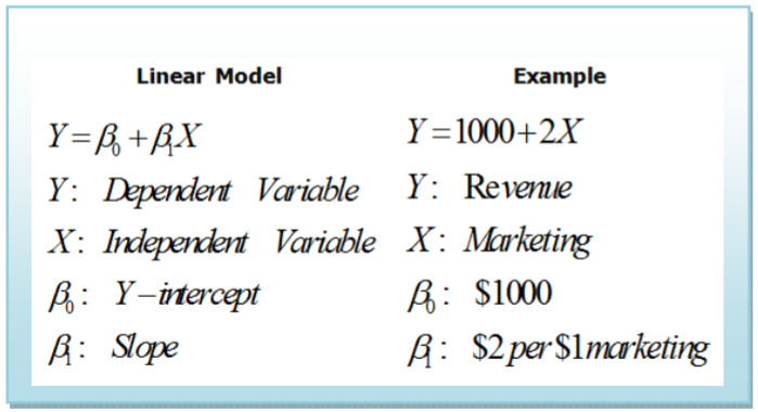
\(Y=\beta_{0}+\beta_{1} X\)
\(Y\): Dependent Variable
\(X\): Independent Variable
\(\beta_{0}\): Y - intercept
\(\beta_{1}\):Slope
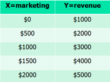
You have a small business producing custom t‐shirts. Without marketing, your business has revenue (sales) of $1000 per week. Every dollar you spend marketing will increase revenue by 2 dollars. Let variable \(X\) represent the amount spent on marketing and let variable \(Y\) represent revenue per week. Write a mathematical model that relates \(X\) to \(Y\).
Solution
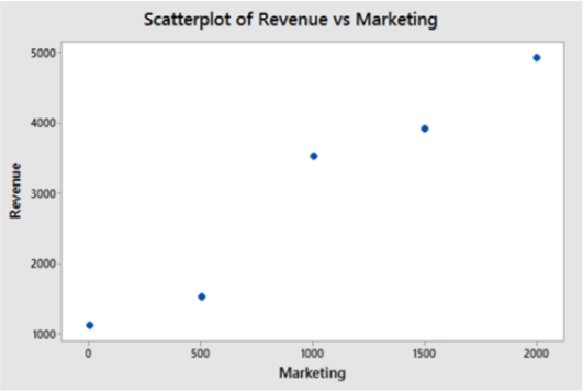
In this example, we are saying that weekly revenue (\(Y\)) depends on marketing expense (\(X\)). $1000 of weekly revenue represents the vertical intercept, and $2 of weekly revenue per $1 marketing represents the slope, or rate of change of the model. We can choose some value of \(X\) and determine \(Y\) and then plot the points on a scatterplot to see this linear relationship.
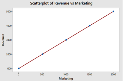
We can then write out the mathematical linear model as an equation:
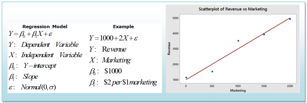
We all learned about these linear models in Algebra classes, but the real world doesn’t generally give such perfect results. In particular, we can choose what to spend on marketing, but the actual revenue will have more uncertainty. For example, the true revenue may look more like this:
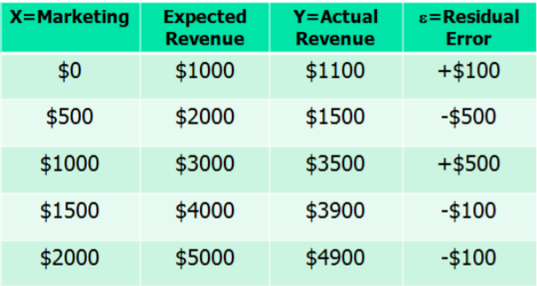
The difference between the actual revenue and the expected revenue is called the residual error, \(\varepsilon\) If we assume that the residual error (represented by \(\varepsilon\)) is a random variable that follows a normal distribution with \(\mu=0\) and \(\sigma\) a constant for all values of \(X\), we have now created a statistical model called a simple linear regression model.