3.6.2: Correlation Coefficient
- Page ID
- 20845
\( \newcommand{\vecs}[1]{\overset { \scriptstyle \rightharpoonup} {\mathbf{#1}} } \)
\( \newcommand{\vecd}[1]{\overset{-\!-\!\rightharpoonup}{\vphantom{a}\smash {#1}}} \)
\( \newcommand{\id}{\mathrm{id}}\) \( \newcommand{\Span}{\mathrm{span}}\)
( \newcommand{\kernel}{\mathrm{null}\,}\) \( \newcommand{\range}{\mathrm{range}\,}\)
\( \newcommand{\RealPart}{\mathrm{Re}}\) \( \newcommand{\ImaginaryPart}{\mathrm{Im}}\)
\( \newcommand{\Argument}{\mathrm{Arg}}\) \( \newcommand{\norm}[1]{\| #1 \|}\)
\( \newcommand{\inner}[2]{\langle #1, #2 \rangle}\)
\( \newcommand{\Span}{\mathrm{span}}\)
\( \newcommand{\id}{\mathrm{id}}\)
\( \newcommand{\Span}{\mathrm{span}}\)
\( \newcommand{\kernel}{\mathrm{null}\,}\)
\( \newcommand{\range}{\mathrm{range}\,}\)
\( \newcommand{\RealPart}{\mathrm{Re}}\)
\( \newcommand{\ImaginaryPart}{\mathrm{Im}}\)
\( \newcommand{\Argument}{\mathrm{Arg}}\)
\( \newcommand{\norm}[1]{\| #1 \|}\)
\( \newcommand{\inner}[2]{\langle #1, #2 \rangle}\)
\( \newcommand{\Span}{\mathrm{span}}\) \( \newcommand{\AA}{\unicode[.8,0]{x212B}}\)
\( \newcommand{\vectorA}[1]{\vec{#1}} % arrow\)
\( \newcommand{\vectorAt}[1]{\vec{\text{#1}}} % arrow\)
\( \newcommand{\vectorB}[1]{\overset { \scriptstyle \rightharpoonup} {\mathbf{#1}} } \)
\( \newcommand{\vectorC}[1]{\textbf{#1}} \)
\( \newcommand{\vectorD}[1]{\overrightarrow{#1}} \)
\( \newcommand{\vectorDt}[1]{\overrightarrow{\text{#1}}} \)
\( \newcommand{\vectE}[1]{\overset{-\!-\!\rightharpoonup}{\vphantom{a}\smash{\mathbf {#1}}}} \)
\( \newcommand{\vecs}[1]{\overset { \scriptstyle \rightharpoonup} {\mathbf{#1}} } \)
\( \newcommand{\vecd}[1]{\overset{-\!-\!\rightharpoonup}{\vphantom{a}\smash {#1}}} \)
\(\newcommand{\avec}{\mathbf a}\) \(\newcommand{\bvec}{\mathbf b}\) \(\newcommand{\cvec}{\mathbf c}\) \(\newcommand{\dvec}{\mathbf d}\) \(\newcommand{\dtil}{\widetilde{\mathbf d}}\) \(\newcommand{\evec}{\mathbf e}\) \(\newcommand{\fvec}{\mathbf f}\) \(\newcommand{\nvec}{\mathbf n}\) \(\newcommand{\pvec}{\mathbf p}\) \(\newcommand{\qvec}{\mathbf q}\) \(\newcommand{\svec}{\mathbf s}\) \(\newcommand{\tvec}{\mathbf t}\) \(\newcommand{\uvec}{\mathbf u}\) \(\newcommand{\vvec}{\mathbf v}\) \(\newcommand{\wvec}{\mathbf w}\) \(\newcommand{\xvec}{\mathbf x}\) \(\newcommand{\yvec}{\mathbf y}\) \(\newcommand{\zvec}{\mathbf z}\) \(\newcommand{\rvec}{\mathbf r}\) \(\newcommand{\mvec}{\mathbf m}\) \(\newcommand{\zerovec}{\mathbf 0}\) \(\newcommand{\onevec}{\mathbf 1}\) \(\newcommand{\real}{\mathbb R}\) \(\newcommand{\twovec}[2]{\left[\begin{array}{r}#1 \\ #2 \end{array}\right]}\) \(\newcommand{\ctwovec}[2]{\left[\begin{array}{c}#1 \\ #2 \end{array}\right]}\) \(\newcommand{\threevec}[3]{\left[\begin{array}{r}#1 \\ #2 \\ #3 \end{array}\right]}\) \(\newcommand{\cthreevec}[3]{\left[\begin{array}{c}#1 \\ #2 \\ #3 \end{array}\right]}\) \(\newcommand{\fourvec}[4]{\left[\begin{array}{r}#1 \\ #2 \\ #3 \\ #4 \end{array}\right]}\) \(\newcommand{\cfourvec}[4]{\left[\begin{array}{c}#1 \\ #2 \\ #3 \\ #4 \end{array}\right]}\) \(\newcommand{\fivevec}[5]{\left[\begin{array}{r}#1 \\ #2 \\ #3 \\ #4 \\ #5 \\ \end{array}\right]}\) \(\newcommand{\cfivevec}[5]{\left[\begin{array}{c}#1 \\ #2 \\ #3 \\ #4 \\ #5 \\ \end{array}\right]}\) \(\newcommand{\mattwo}[4]{\left[\begin{array}{rr}#1 \amp #2 \\ #3 \amp #4 \\ \end{array}\right]}\) \(\newcommand{\laspan}[1]{\text{Span}\{#1\}}\) \(\newcommand{\bcal}{\cal B}\) \(\newcommand{\ccal}{\cal C}\) \(\newcommand{\scal}{\cal S}\) \(\newcommand{\wcal}{\cal W}\) \(\newcommand{\ecal}{\cal E}\) \(\newcommand{\coords}[2]{\left\{#1\right\}_{#2}}\) \(\newcommand{\gray}[1]{\color{gray}{#1}}\) \(\newcommand{\lgray}[1]{\color{lightgray}{#1}}\) \(\newcommand{\rank}{\operatorname{rank}}\) \(\newcommand{\row}{\text{Row}}\) \(\newcommand{\col}{\text{Col}}\) \(\renewcommand{\row}{\text{Row}}\) \(\newcommand{\nul}{\text{Nul}}\) \(\newcommand{\var}{\text{Var}}\) \(\newcommand{\corr}{\text{corr}}\) \(\newcommand{\len}[1]{\left|#1\right|}\) \(\newcommand{\bbar}{\overline{\bvec}}\) \(\newcommand{\bhat}{\widehat{\bvec}}\) \(\newcommand{\bperp}{\bvec^\perp}\) \(\newcommand{\xhat}{\widehat{\xvec}}\) \(\newcommand{\vhat}{\widehat{\vvec}}\) \(\newcommand{\uhat}{\widehat{\uvec}}\) \(\newcommand{\what}{\widehat{\wvec}}\) \(\newcommand{\Sighat}{\widehat{\Sigma}}\) \(\newcommand{\lt}{<}\) \(\newcommand{\gt}{>}\) \(\newcommand{\amp}{&}\) \(\definecolor{fillinmathshade}{gray}{0.9}\)
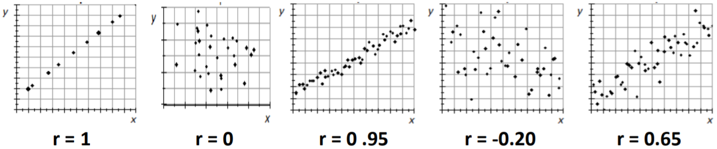
The correlation coefficient (represented by the letter \(r\)) measures both the direction and strength of a linear relationship or association between two variables. The value \(r\) will always take on a value between ‐1 and 1. Values close to zero indicate a very weak correlation. Values close to 1 or ‐1 indicate a very strong correlation. The correlation coefficient should not be used for non‐linear correlation.
It is important to ignore the sign when determining strength of correlation. For example, \(r = ‐0.75\) would indicate a stronger correlation than \(r = 0.62\), since ‐0.75 is farther from zero.
We will use technology to calculate the correlation coefficient, but formulas for manually calculating \(r\) are presented at the end of this section.
Interpreting the correlation coefficient (\(r\))
\[-1 \leq r \leq 1 \nonumber \]
\(r = 1\) means perfect positive correlation
\(r = ‐1\) means perfect negative correlation
\(r = 0\) mean no correlation
The farther \(r\) is from zero, the stronger the correlation
\(r > 0\) means positive correlation
\(r < 0\) means negative correlation
Some Examples
Example: Cucumber yield and rainfall
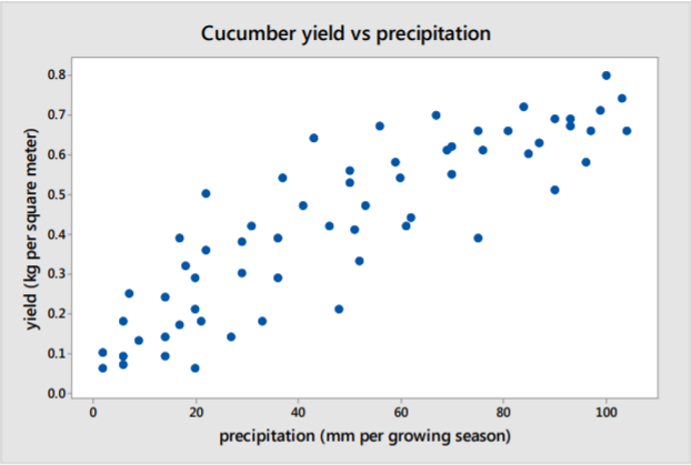
This scatterplot represents randomly collected data on growing season precipitation and cucumber yield.
\(r= 0.871\) indicating strong positive correlation.
Example: GPA and missing class
A group of students at Georgia College conducted a survey asking random students various questions about their academic profile. One part of their study was to see if there is any correlation between various students’ GPA and classes missed.
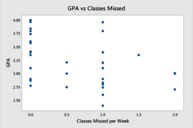
\(r= ‐0.236\) indicating weak negative correlation.
Example: Commute times and temperature
A mathematics instructor commutes by car from his home in San Francisco to De Anza College in Cupertino, California. For 100 randomly selected days during the year, the instructor recorded the commuting time and the temperature in Cupertino at time of arrival.
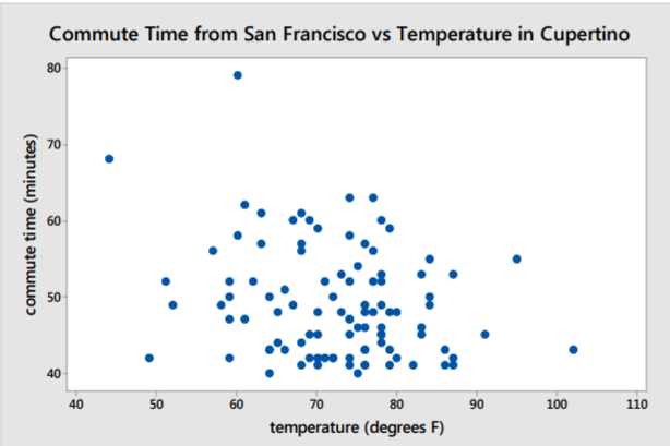
\(r = ‐0.02\) indicating no correlation.
Calculating the correlation coefficient
Manually calculating the correlation coefficient is a tedious process, but the needed formulas and one simple example are presented here:
Formulas for calculating the correlation coefficient (\(r\))
\[r=\dfrac{S S X Y}{\sqrt{S S X \cdot S S Y}} \nonumber \]
\[S S X=\Sigma X^{2}-\dfrac{1}{n}(\Sigma X)^{2} \nonumber \]
\[S S Y=\Sigma Y^{2}-\dfrac{1}{n}(\Sigma Y)^{2} \nonumber \]
\[S S X Y=\Sigma X Y-\dfrac{1}{n}(\Sigma X \cdot \Sigma Y) \nonumber \]
Example: Sunglasses sales and rainfall
A company selling sunglasses determined the units sold per 1000 people and the annual rainfall in 5 cities.
X = rainfall in inches
Y = sales of sunglasses per 1000 people.
X | Y |
---|---|
10 | 40 |
15 | 35 |
20 | 25 |
30 | 25 |
40 | 15 |
Solution
First, find the following sums:
\[\sum X, \sum Y, \sum X^{2}, \sum Y^{2}, \sum X Y \nonumber \]
\(X)\) | \(Y\) | \(X^{2}\) | \(Y^{2}\) | \(XY\) | |
---|---|---|---|---|---|
10 | 40 | 100 | 1600 | 400 | |
15 | 35 | 225 | 1225 | 525 | |
20 | 25 | 400 | 625 | 500 | |
30 | 25 | 900 | 625 | 750 | |
40 | 15 | 1600 | 225 | 600 | |
\(\mathbf{\Sigma}\) | 115 | 140 | 3225 | 4300 | 2775 |
Then, find \(SSX\), \(SSY\), \(SSXY\)
\(\begin{array}{ll}
S S X=3225-115^{2} / 5 & =580 \\
S S Y=4300-140^{2} / 5 & =380 \\
S S X Y=2775-(115)(140) / 5 & =-445
\end{array}\)
Finally, calculate \(r\)
\(r=\dfrac{S S X Y}{\sqrt{S S X \cdot S S Y}}=\dfrac{-445}{\sqrt{580 \cdot 330}}=-0.9479\)
The correlation coefficient is ‐0.95, indicating a strong, negative correlation between rainfall and sales of sunglasses.