10.2: R and time
- Page ID
- 3611
\( \newcommand{\vecs}[1]{\overset { \scriptstyle \rightharpoonup} {\mathbf{#1}} } \)
\( \newcommand{\vecd}[1]{\overset{-\!-\!\rightharpoonup}{\vphantom{a}\smash {#1}}} \)
\( \newcommand{\id}{\mathrm{id}}\) \( \newcommand{\Span}{\mathrm{span}}\)
( \newcommand{\kernel}{\mathrm{null}\,}\) \( \newcommand{\range}{\mathrm{range}\,}\)
\( \newcommand{\RealPart}{\mathrm{Re}}\) \( \newcommand{\ImaginaryPart}{\mathrm{Im}}\)
\( \newcommand{\Argument}{\mathrm{Arg}}\) \( \newcommand{\norm}[1]{\| #1 \|}\)
\( \newcommand{\inner}[2]{\langle #1, #2 \rangle}\)
\( \newcommand{\Span}{\mathrm{span}}\)
\( \newcommand{\id}{\mathrm{id}}\)
\( \newcommand{\Span}{\mathrm{span}}\)
\( \newcommand{\kernel}{\mathrm{null}\,}\)
\( \newcommand{\range}{\mathrm{range}\,}\)
\( \newcommand{\RealPart}{\mathrm{Re}}\)
\( \newcommand{\ImaginaryPart}{\mathrm{Im}}\)
\( \newcommand{\Argument}{\mathrm{Arg}}\)
\( \newcommand{\norm}[1]{\| #1 \|}\)
\( \newcommand{\inner}[2]{\langle #1, #2 \rangle}\)
\( \newcommand{\Span}{\mathrm{span}}\) \( \newcommand{\AA}{\unicode[.8,0]{x212B}}\)
\( \newcommand{\vectorA}[1]{\vec{#1}} % arrow\)
\( \newcommand{\vectorAt}[1]{\vec{\text{#1}}} % arrow\)
\( \newcommand{\vectorB}[1]{\overset { \scriptstyle \rightharpoonup} {\mathbf{#1}} } \)
\( \newcommand{\vectorC}[1]{\textbf{#1}} \)
\( \newcommand{\vectorD}[1]{\overrightarrow{#1}} \)
\( \newcommand{\vectorDt}[1]{\overrightarrow{\text{#1}}} \)
\( \newcommand{\vectE}[1]{\overset{-\!-\!\rightharpoonup}{\vphantom{a}\smash{\mathbf {#1}}}} \)
\( \newcommand{\vecs}[1]{\overset { \scriptstyle \rightharpoonup} {\mathbf{#1}} } \)
\( \newcommand{\vecd}[1]{\overset{-\!-\!\rightharpoonup}{\vphantom{a}\smash {#1}}} \)
\(\newcommand{\avec}{\mathbf a}\) \(\newcommand{\bvec}{\mathbf b}\) \(\newcommand{\cvec}{\mathbf c}\) \(\newcommand{\dvec}{\mathbf d}\) \(\newcommand{\dtil}{\widetilde{\mathbf d}}\) \(\newcommand{\evec}{\mathbf e}\) \(\newcommand{\fvec}{\mathbf f}\) \(\newcommand{\nvec}{\mathbf n}\) \(\newcommand{\pvec}{\mathbf p}\) \(\newcommand{\qvec}{\mathbf q}\) \(\newcommand{\svec}{\mathbf s}\) \(\newcommand{\tvec}{\mathbf t}\) \(\newcommand{\uvec}{\mathbf u}\) \(\newcommand{\vvec}{\mathbf v}\) \(\newcommand{\wvec}{\mathbf w}\) \(\newcommand{\xvec}{\mathbf x}\) \(\newcommand{\yvec}{\mathbf y}\) \(\newcommand{\zvec}{\mathbf z}\) \(\newcommand{\rvec}{\mathbf r}\) \(\newcommand{\mvec}{\mathbf m}\) \(\newcommand{\zerovec}{\mathbf 0}\) \(\newcommand{\onevec}{\mathbf 1}\) \(\newcommand{\real}{\mathbb R}\) \(\newcommand{\twovec}[2]{\left[\begin{array}{r}#1 \\ #2 \end{array}\right]}\) \(\newcommand{\ctwovec}[2]{\left[\begin{array}{c}#1 \\ #2 \end{array}\right]}\) \(\newcommand{\threevec}[3]{\left[\begin{array}{r}#1 \\ #2 \\ #3 \end{array}\right]}\) \(\newcommand{\cthreevec}[3]{\left[\begin{array}{c}#1 \\ #2 \\ #3 \end{array}\right]}\) \(\newcommand{\fourvec}[4]{\left[\begin{array}{r}#1 \\ #2 \\ #3 \\ #4 \end{array}\right]}\) \(\newcommand{\cfourvec}[4]{\left[\begin{array}{c}#1 \\ #2 \\ #3 \\ #4 \end{array}\right]}\) \(\newcommand{\fivevec}[5]{\left[\begin{array}{r}#1 \\ #2 \\ #3 \\ #4 \\ #5 \\ \end{array}\right]}\) \(\newcommand{\cfivevec}[5]{\left[\begin{array}{c}#1 \\ #2 \\ #3 \\ #4 \\ #5 \\ \end{array}\right]}\) \(\newcommand{\mattwo}[4]{\left[\begin{array}{rr}#1 \amp #2 \\ #3 \amp #4 \\ \end{array}\right]}\) \(\newcommand{\laspan}[1]{\text{Span}\{#1\}}\) \(\newcommand{\bcal}{\cal B}\) \(\newcommand{\ccal}{\cal C}\) \(\newcommand{\scal}{\cal S}\) \(\newcommand{\wcal}{\cal W}\) \(\newcommand{\ecal}{\cal E}\) \(\newcommand{\coords}[2]{\left\{#1\right\}_{#2}}\) \(\newcommand{\gray}[1]{\color{gray}{#1}}\) \(\newcommand{\lgray}[1]{\color{lightgray}{#1}}\) \(\newcommand{\rank}{\operatorname{rank}}\) \(\newcommand{\row}{\text{Row}}\) \(\newcommand{\col}{\text{Col}}\) \(\renewcommand{\row}{\text{Row}}\) \(\newcommand{\nul}{\text{Nul}}\) \(\newcommand{\var}{\text{Var}}\) \(\newcommand{\corr}{\text{corr}}\) \(\newcommand{\len}[1]{\left|#1\right|}\) \(\newcommand{\bbar}{\overline{\bvec}}\) \(\newcommand{\bhat}{\widehat{\bvec}}\) \(\newcommand{\bperp}{\bvec^\perp}\) \(\newcommand{\xhat}{\widehat{\xvec}}\) \(\newcommand{\vhat}{\widehat{\vvec}}\) \(\newcommand{\uhat}{\widehat{\uvec}}\) \(\newcommand{\what}{\widehat{\wvec}}\) \(\newcommand{\Sighat}{\widehat{\Sigma}}\) \(\newcommand{\lt}{<}\) \(\newcommand{\gt}{>}\) \(\newcommand{\amp}{&}\) \(\definecolor{fillinmathshade}{gray}{0.9}\)If we measure same object multiple times, especially at regular (sampling) intervals, we will finally have the time series, specific type of measurement data. While many common options of data analysis are applicable to time series, there are multiple specific methods and plots.
Time series frequently have two components, non-random and random. The first could in turn contain the seasonal component which is related with time periodically, like year seasons or day and night. The trend is the second part of non-random component, it is both no-random and non-periodical.
If time series has the non-random component, the later values should correlate with earlier values. This is autocorrelation. Autocorrelation has lags, intervals of time where correlation is maximal. These lags could be organized hierarchically.
Different time series could be cross-correlated if they are related.
If the goal is to analyze the time series and (1) fill the gaps within (interpolation) or (2) make forecast (extrapolation), then one need to create the time series model (for example, with arima() function).
But before the start, one will need to convert the ordinary data frame or vector into time series. Conversion of dates is probably most complicated:
Code \(\PageIndex{1}\) (R):
In that example, we showed how to use as.Data() function to convert one type to another. Actually, our recommendation is to use the fully numerical date:
Code \(\PageIndex{2}\) (R):
The advantage of this system is that dates here are accessible (for example, for sorting) both as numbers and as dates.
And here is how to create time series of the regular type:
Code \(\PageIndex{3}\) (R):
(If the time series is irregular, one may want to apply its() from the its package.)
It is possible to convert the whole matrix. In that case, every column will become the time series:
Code \(\PageIndex{4}\) (R):
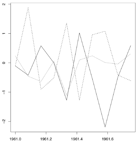
Generic plot() function “knows” how to show the time series (Figure \(\PageIndex{1}\):
Code \(\PageIndex{5}\) (R):
(There is also specialized ts.plot() function.)

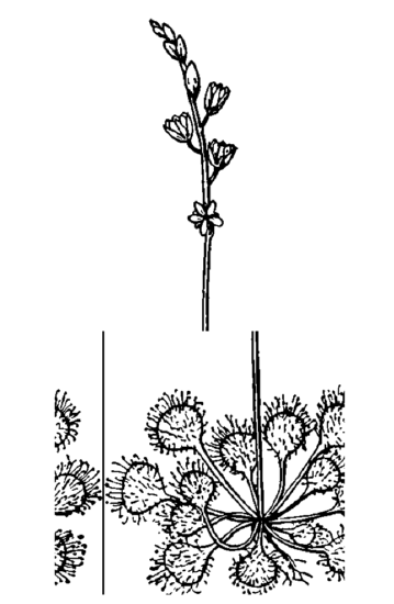
There are numerous analytical methods applicable to time series. We will show some of them on the example of “non-stop” observations on carnivorous plant—sundew (Drosera rotundifolia). In nature, leaves of sundew are constantly open and close in hope to catch and then digest the insect prey (Figure \(\PageIndex{2}\)). File sundew.txt contains results of observations related with the fourth leaf of the second plant in the group observed. The leaf condition was noted every 40 minutes, and there were 36 observations per 24 hours. We will try to make the time series from SHAPE column which encodes the shape of leaf blade (1 flat, 2 concave), it is the ranked data since it is possible to imagine the SHAPE \(= 1.5\). Command file.show() reveals this structure:

WET;SHAPE
2;1
1;1
1;1
...
Now we can read the file and check it:
Code \(\PageIndex{6}\) (R):
Everything looks fine, there are no visible errors or outliers. Now convert the SHAPE variable into time series:
Code \(\PageIndex{7}\) (R):
Let us check it:
Code \(\PageIndex{8}\) (R):
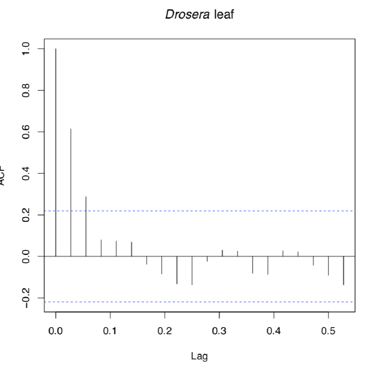
Looks perfect because our observations lasted for slightly more than 3 days. Now access the periodicity of the time series (seasonal component) and check out the possible trend (Figure \(\PageIndex{3}\)):
Code \(\PageIndex{9}\) (R):
(Please note also how expression() was used to make part of the title italic, like it is traditional in biology.)
Command acf() (auto-correlation function) outputs coefficients of autocorrelation and also draws the autocorrelation plot. In our case, significant periodicity is absent because almost all pikes lay within the confidence interval. Only first tree pikes are outside, these correspond with lags lower than 0.05 day (about 1 hour or less). It means that within one hour, the leaf shape will stay the same. On larger intervals (we have 24 h period), these predictions are not quite possible.

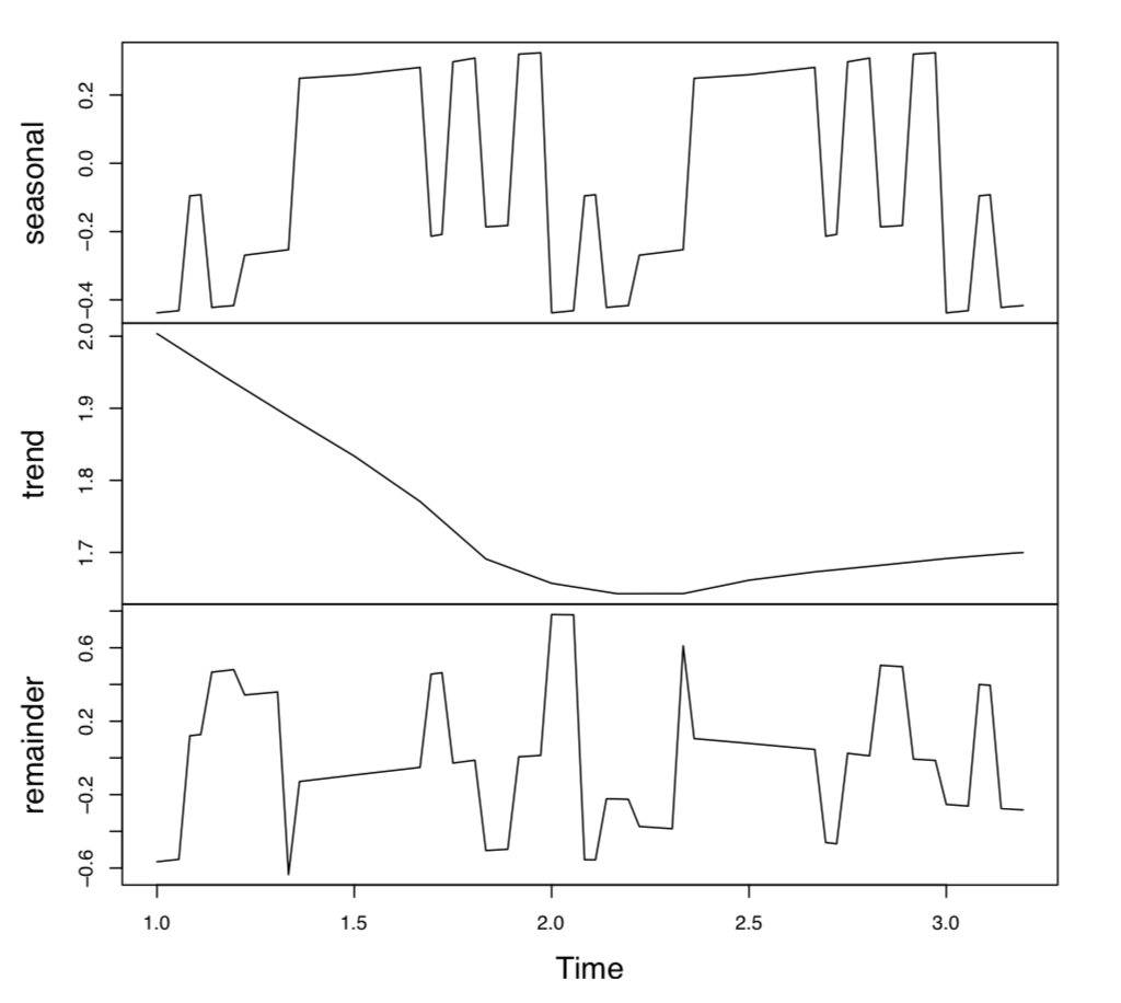
However, there is a tendency in pikes: they are much smaller to the right. It could be the sign of trend. Check it (Figure \(\PageIndex{4}\)):
Code \(\PageIndex{10}\) (R):
As you see, there is a tendency for decreasing of SHAPE with time. We used stl() function (STL—“Seasonal Decomposition of Time Series by Loess” to show that. STL segregates the time series into seasonal (day length in our case), random and trend components.
WET is the second character in our sundew dataset. It shows the wetness of the leaf. Does wetness have the same periodicity and trend as the leaf shape?


