7.4: Semi-supervised learning

Last updated
Save as PDF

Page ID: 3585

\( \newcommand{\vecs}[1]{\overset { \scriptstyle \rightharpoonup} {\mathbf{#1}} } \) \( \newcommand{\vecd}[1]{\overset{-\!-\!\rightharpoonup}{\vphantom{a}\smash {#1}}} \)\(\newcommand{\id}{\mathrm{id}}\) \( \newcommand{\Span}{\mathrm{span}}\) \( \newcommand{\kernel}{\mathrm{null}\,}\) \( \newcommand{\range}{\mathrm{range}\,}\) \( \newcommand{\RealPart}{\mathrm{Re}}\) \( \newcommand{\ImaginaryPart}{\mathrm{Im}}\) \( \newcommand{\Argument}{\mathrm{Arg}}\) \( \newcommand{\norm}[1]{\| #1 \|}\) \( \newcommand{\inner}[2]{\langle #1, #2 \rangle}\) \( \newcommand{\Span}{\mathrm{span}}\) \(\newcommand{\id}{\mathrm{id}}\) \( \newcommand{\Span}{\mathrm{span}}\) \( \newcommand{\kernel}{\mathrm{null}\,}\) \( \newcommand{\range}{\mathrm{range}\,}\) \( \newcommand{\RealPart}{\mathrm{Re}}\) \( \newcommand{\ImaginaryPart}{\mathrm{Im}}\) \( \newcommand{\Argument}{\mathrm{Arg}}\) \( \newcommand{\norm}[1]{\| #1 \|}\) \( \newcommand{\inner}[2]{\langle #1, #2 \rangle}\) \( \newcommand{\Span}{\mathrm{span}}\)\(\newcommand{\AA}{\unicode[.8,0]{x212B}}\)

There is no deep distinction between supervised and non-supevised methods, some of non-supervised (like SOM or PCA) could use training whereas some supervised (LDA, Random Forest, recursive partitioning) are useful directly as visualizations.

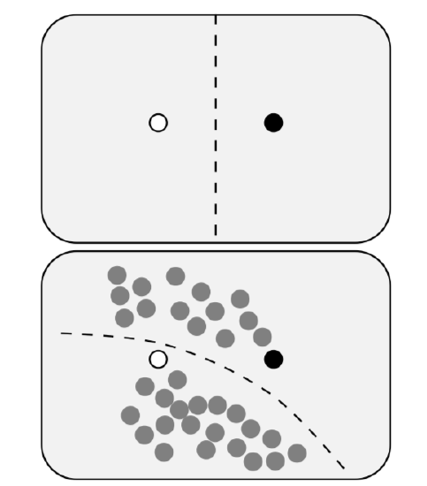
And there is a in-between semi-supervised learning. It takes into account both data features and data labeling (Figure \(\PageIndex{2}\)).

One of the most important features of SSL is an ability to work with the very small training sample. Many really bright ideas are embedded in SSL, here we illustrate two of them. Self-learning is when classification is developed in multiple cycles. On each cycle, testing points which are most confident, are labeled and added to the training set:

Screen Shot 2019-01-26 at 1.23.22 AM.png — Figure \(\PageIndex{1}\) The neural network.

Code \(\PageIndex{1}\) (R):

library(SSL)
iris.30 <- seq(1, nrow(iris), 30) # only 5 labeled points!
iris.sslt1 <- sslSelfTrain(iris[iris.30, -5], iris[iris.30, 5], iris[-iris.30, -5], nrounds=20, n=5) # n found manually, ignore errors while searching
iris.sslt2 <- levels(iris$Species)[iris.sslt1]
Misclass(iris.sslt2, iris[-iris.30, 5])

Screen Shot 2019-01-26 at 1.25.28 AM.png — Figure \(\PageIndex{2}\) How semi-supervised learning can improve learning results. If only labeled data used, then the most logical split is between labeled points. However, if we look on the testing set, it become apparent that training points are parts of more complicated structures, and the actual split goes in the other direction.

As you see, with only 5 data points (approximately 3% of data vs. 33% of data in iris.train), semi-supervised self-leaning (based on gradient boosting in this case) reached 73% of accuracy.

Another semi-supervised approach is based on graph theory and uses graph label propagation:

Code \(\PageIndex{2}\) (R):

iris.10 <- seq(1, nrow(iris), 10) # 10 labeled points
iris.sslp1 <- sslLabelProp(iris[, -5], iris[iris.10, 5], iris.10, graph.type="knn", k=30) # k found manually
iris.sslp2 <- ifelse(round(iris.sslp1) == 0, 1, round(iris.sslp1)) ## "practice is when everything works but nobody knows why..."
iris.sslp3 <- levels(iris$Species)[iris.sslp2]
Misclass(iris.sslp3[-iris.10], iris[-iris.10, 5])

The idea of this algorithm is similar to what was shown on the illustration (Figure \(\PageIndex{2}\)) above. Label propagation with 10 points outperforms Randon Forest (see above) which used 30 points.