8.6: The Simplest Model- The Mean

Last updated
Save as PDF

Page ID: 8752

\( \newcommand{\vecs}[1]{\overset { \scriptstyle \rightharpoonup} {\mathbf{#1}} } \) \( \newcommand{\vecd}[1]{\overset{-\!-\!\rightharpoonup}{\vphantom{a}\smash {#1}}} \)\(\newcommand{\id}{\mathrm{id}}\) \( \newcommand{\Span}{\mathrm{span}}\) \( \newcommand{\kernel}{\mathrm{null}\,}\) \( \newcommand{\range}{\mathrm{range}\,}\) \( \newcommand{\RealPart}{\mathrm{Re}}\) \( \newcommand{\ImaginaryPart}{\mathrm{Im}}\) \( \newcommand{\Argument}{\mathrm{Arg}}\) \( \newcommand{\norm}[1]{\| #1 \|}\) \( \newcommand{\inner}[2]{\langle #1, #2 \rangle}\) \( \newcommand{\Span}{\mathrm{span}}\) \(\newcommand{\id}{\mathrm{id}}\) \( \newcommand{\Span}{\mathrm{span}}\) \( \newcommand{\kernel}{\mathrm{null}\,}\) \( \newcommand{\range}{\mathrm{range}\,}\) \( \newcommand{\RealPart}{\mathrm{Re}}\) \( \newcommand{\ImaginaryPart}{\mathrm{Im}}\) \( \newcommand{\Argument}{\mathrm{Arg}}\) \( \newcommand{\norm}[1]{\| #1 \|}\) \( \newcommand{\inner}[2]{\langle #1, #2 \rangle}\) \( \newcommand{\Span}{\mathrm{span}}\)\(\newcommand{\AA}{\unicode[.8,0]{x212B}}\)

We have already encountered the mean (or average), and in fact most people know about the average even if they have never taken a statistics class. It is commonly used to describe what we call the “central tendency” of a dataset – that is, what value are the data centered around? Most people don’t think of computing a mean as fitting a model to data. However, that’s exactly what we are doing when we compute the mean.

We have already seen the formula for computing the mean of a sample of data:

\(\ \bar{X}=\frac{{\sum_{i=1}^n}x_i}{n}\)

Note that I said that this formula was specifically for a sample of data, which is a set of data points selected from a larger population. Using a sample, we wish to characterize a larger population – the full set of individuals that we are interested in. For example, if we are a political pollster our population of interest might be all registered voters, whereas our sample might just include a few thousand people sampled from this population. Later in the course we will talk in more detail about sampling, but for now the important point is that statisticians generally like to use different symbols to differentiate statistics that describe values for a sample from parameters that describe the true values for a population; in this case, the formula for the population mean (denoted as μ) is:

\(\ \mu=\frac{\sum_{i=1}^Nx_i}{N}\)

where N is the size of the entire population.

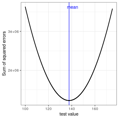
We have already seen that the mean is the summary statistic that is guaranteed to give us a mean error of zero. The mean also has another characteristic: It is the summary statistic that has the lowest possible value for the sum of squared errors (SSE). In statistics, we refer to this as being the “best” estimator. We could prove this mathematically, but instead we will demonstrate it graphically in Figure 8.7.

Figure 8.7: A demonstration of the mean as the statistic that minimizes the sum of squared errors. Using the NHANES child height data, we compute the mean (denoted by the blue bar). Then, we test a range of other values, and for each one we compute the sum of squared errors for each data point from that value, which are denoted by the black curve. We see that the mean falls at the minimum of the squared error plot.

This minimization of SSE is a good feature, and it’s why the mean is the most commonly used statistic to summarize data. However, the mean also has a dark side. Let’s say that five people are in a bar, and we examine each person’s income:

Table 8.1: Income for our five bar patrons
income	person
48000	Joe
64000	Karen
58000	Mark
72000	Andrea
66000	Pat

The mean (61600.00) seems to be a pretty good summary of the income of those five people. Now let’s look at what happens if Beyoncé Knowles walks into the bar:

Table 8.2: Income for our five bar patrons plus Beyoncé Knowles.
income	person
4.8e+04	Joe
6.4e+04	Karen
5.8e+04	Mark
7.2e+04	Andrea
6.6e+04	Pat
5.4e+07	Beyonce

The mean is now almost 10 million dollars, which is not really representative of any of the people in the bar – in particular, it is heavily driven by the outlying value of Beyoncé. In general, the mean is highly sensitive to extreme values, which is why it’s always important to ensure that there are no extreme values when using the mean to summarize data.

8.5.1 The median

If we want to summarize the data in a way that is less sensitive to outliers, we can use another statistic called the median. If we were to sort all of the values in order of their magnitude, then the median is the value in the middle. If there is an even number of values then there will be two values tied for the middle place, in which case we take the mean (i.e. the halfway point) of those two numbers.

Let’s look at an example. Say we want to summarize the following values:

8  6  3 14 12  7  6  4  9

If we sort those values:

3  4  6  6  7  8  9 12 14

Then the median is the middle value – in this case, the 5th of the 9 values.

Whereas the mean minimizes the sum of squared errors, the median minimizes a slighty different quantity: The sum of absolute errors. This explains why it is less sensitive to outliers – squaring is going to exacerbate the effect of large errors compared to taking the absolute value. We can see this in the case of the income example: The median is much more representative of the group as a whole, and less sensitive to the one large outlier.

Table 8.3: Summary statistics for income after arrival of Beyoncé Knowles.
Statistic	Value
Mean	9051333
Median	65000

Given this, why would we ever use the mean? As we will see in a later chapter, the mean is the “best” estimator in the sense that it will vary less from sample to sample compared to other estimators. It’s up to us to decide whether that is worth the sensitivity to potential outliers – statistics is all about tradeoffs.