4.3: Random Variables
- Page ID
- 7806
\( \newcommand{\vecs}[1]{\overset { \scriptstyle \rightharpoonup} {\mathbf{#1}} } \)
\( \newcommand{\vecd}[1]{\overset{-\!-\!\rightharpoonup}{\vphantom{a}\smash {#1}}} \)
\( \newcommand{\dsum}{\displaystyle\sum\limits} \)
\( \newcommand{\dint}{\displaystyle\int\limits} \)
\( \newcommand{\dlim}{\displaystyle\lim\limits} \)
\( \newcommand{\id}{\mathrm{id}}\) \( \newcommand{\Span}{\mathrm{span}}\)
( \newcommand{\kernel}{\mathrm{null}\,}\) \( \newcommand{\range}{\mathrm{range}\,}\)
\( \newcommand{\RealPart}{\mathrm{Re}}\) \( \newcommand{\ImaginaryPart}{\mathrm{Im}}\)
\( \newcommand{\Argument}{\mathrm{Arg}}\) \( \newcommand{\norm}[1]{\| #1 \|}\)
\( \newcommand{\inner}[2]{\langle #1, #2 \rangle}\)
\( \newcommand{\Span}{\mathrm{span}}\)
\( \newcommand{\id}{\mathrm{id}}\)
\( \newcommand{\Span}{\mathrm{span}}\)
\( \newcommand{\kernel}{\mathrm{null}\,}\)
\( \newcommand{\range}{\mathrm{range}\,}\)
\( \newcommand{\RealPart}{\mathrm{Re}}\)
\( \newcommand{\ImaginaryPart}{\mathrm{Im}}\)
\( \newcommand{\Argument}{\mathrm{Arg}}\)
\( \newcommand{\norm}[1]{\| #1 \|}\)
\( \newcommand{\inner}[2]{\langle #1, #2 \rangle}\)
\( \newcommand{\Span}{\mathrm{span}}\) \( \newcommand{\AA}{\unicode[.8,0]{x212B}}\)
\( \newcommand{\vectorA}[1]{\vec{#1}} % arrow\)
\( \newcommand{\vectorAt}[1]{\vec{\text{#1}}} % arrow\)
\( \newcommand{\vectorB}[1]{\overset { \scriptstyle \rightharpoonup} {\mathbf{#1}} } \)
\( \newcommand{\vectorC}[1]{\textbf{#1}} \)
\( \newcommand{\vectorD}[1]{\overrightarrow{#1}} \)
\( \newcommand{\vectorDt}[1]{\overrightarrow{\text{#1}}} \)
\( \newcommand{\vectE}[1]{\overset{-\!-\!\rightharpoonup}{\vphantom{a}\smash{\mathbf {#1}}}} \)
\( \newcommand{\vecs}[1]{\overset { \scriptstyle \rightharpoonup} {\mathbf{#1}} } \)
\( \newcommand{\vecd}[1]{\overset{-\!-\!\rightharpoonup}{\vphantom{a}\smash {#1}}} \)
\(\newcommand{\avec}{\mathbf a}\) \(\newcommand{\bvec}{\mathbf b}\) \(\newcommand{\cvec}{\mathbf c}\) \(\newcommand{\dvec}{\mathbf d}\) \(\newcommand{\dtil}{\widetilde{\mathbf d}}\) \(\newcommand{\evec}{\mathbf e}\) \(\newcommand{\fvec}{\mathbf f}\) \(\newcommand{\nvec}{\mathbf n}\) \(\newcommand{\pvec}{\mathbf p}\) \(\newcommand{\qvec}{\mathbf q}\) \(\newcommand{\svec}{\mathbf s}\) \(\newcommand{\tvec}{\mathbf t}\) \(\newcommand{\uvec}{\mathbf u}\) \(\newcommand{\vvec}{\mathbf v}\) \(\newcommand{\wvec}{\mathbf w}\) \(\newcommand{\xvec}{\mathbf x}\) \(\newcommand{\yvec}{\mathbf y}\) \(\newcommand{\zvec}{\mathbf z}\) \(\newcommand{\rvec}{\mathbf r}\) \(\newcommand{\mvec}{\mathbf m}\) \(\newcommand{\zerovec}{\mathbf 0}\) \(\newcommand{\onevec}{\mathbf 1}\) \(\newcommand{\real}{\mathbb R}\) \(\newcommand{\twovec}[2]{\left[\begin{array}{r}#1 \\ #2 \end{array}\right]}\) \(\newcommand{\ctwovec}[2]{\left[\begin{array}{c}#1 \\ #2 \end{array}\right]}\) \(\newcommand{\threevec}[3]{\left[\begin{array}{r}#1 \\ #2 \\ #3 \end{array}\right]}\) \(\newcommand{\cthreevec}[3]{\left[\begin{array}{c}#1 \\ #2 \\ #3 \end{array}\right]}\) \(\newcommand{\fourvec}[4]{\left[\begin{array}{r}#1 \\ #2 \\ #3 \\ #4 \end{array}\right]}\) \(\newcommand{\cfourvec}[4]{\left[\begin{array}{c}#1 \\ #2 \\ #3 \\ #4 \end{array}\right]}\) \(\newcommand{\fivevec}[5]{\left[\begin{array}{r}#1 \\ #2 \\ #3 \\ #4 \\ #5 \\ \end{array}\right]}\) \(\newcommand{\cfivevec}[5]{\left[\begin{array}{c}#1 \\ #2 \\ #3 \\ #4 \\ #5 \\ \end{array}\right]}\) \(\newcommand{\mattwo}[4]{\left[\begin{array}{rr}#1 \amp #2 \\ #3 \amp #4 \\ \end{array}\right]}\) \(\newcommand{\laspan}[1]{\text{Span}\{#1\}}\) \(\newcommand{\bcal}{\cal B}\) \(\newcommand{\ccal}{\cal C}\) \(\newcommand{\scal}{\cal S}\) \(\newcommand{\wcal}{\cal W}\) \(\newcommand{\ecal}{\cal E}\) \(\newcommand{\coords}[2]{\left\{#1\right\}_{#2}}\) \(\newcommand{\gray}[1]{\color{gray}{#1}}\) \(\newcommand{\lgray}[1]{\color{lightgray}{#1}}\) \(\newcommand{\rank}{\operatorname{rank}}\) \(\newcommand{\row}{\text{Row}}\) \(\newcommand{\col}{\text{Col}}\) \(\renewcommand{\row}{\text{Row}}\) \(\newcommand{\nul}{\text{Nul}}\) \(\newcommand{\var}{\text{Var}}\) \(\newcommand{\corr}{\text{corr}}\) \(\newcommand{\len}[1]{\left|#1\right|}\) \(\newcommand{\bbar}{\overline{\bvec}}\) \(\newcommand{\bhat}{\widehat{\bvec}}\) \(\newcommand{\bperp}{\bvec^\perp}\) \(\newcommand{\xhat}{\widehat{\xvec}}\) \(\newcommand{\vhat}{\widehat{\vvec}}\) \(\newcommand{\uhat}{\widehat{\uvec}}\) \(\newcommand{\what}{\widehat{\wvec}}\) \(\newcommand{\Sighat}{\widehat{\Sigma}}\) \(\newcommand{\lt}{<}\) \(\newcommand{\gt}{>}\) \(\newcommand{\amp}{&}\) \(\definecolor{fillinmathshade}{gray}{0.9}\)Definition and First Examples
Suppose we are doing a random experiment and there is some consequence of the result in which we are interested that can be measured by a number. The experiment might be playing a game of chance and the result could be how much you win or lose depending upon the outcome, or the experiment could be which part of the drives’ manual you randomly choose to study and the result how many points we get on the driver’s license test we make the next day, or the experiment might be giving a new drug to a random patient in medical study and the result would be some medical measurement you make after treatment (blood pressure, white blood cell count, whatever), etc. There is a name for this situation in mathematics
DEFINITION 4.3.1. A choice of a number for each outcome of a random experiment is called a random variable [RV]. If the values an RV takes can be counted, because they are either finite or countably infinite8 in number, the RV is called discrete; if, instead, the RV takes on all the values in an interval of real numbers, the RV is called continuous.
We usually use capital letters to denote RVs and the corresponding lowercase letter to indicate a particular numerical value the RV might have, like \(X\) and \(x\).
EXAMPLE 4.3.2. Suppose we play a silly game where you pay me $5 to play, then I flip a fair coin and I give you $10 if the coin comes up heads and $0 if it comes up tails. Then your net winnings, which would be +$5 or -$5 each time you play, are a random variable. Having only two possible values, this RV is certainly discrete.
EXAMPLE 4.3.3. Weather phenomena vary so much, due to such small effects – such as the famous butterfly flapping its wings in the Amazon rain forest causing a hurricane in North America – that they appear to be a random phenomenon. Therefore, observing the temperature at some weather station is a continuous random variable whose value can be any real number in some range like \(-100\) to \(100\) (we’re doing science, so we use \({}^\circ C\)).
EXAMPLE 4.3.4. Suppose we look at the “roll two fair dice independently” experiment from Example 4.2.7 and Example 4.1.21, which was based on the probability model in Example 4.1.21 and sample space in Example 4.1.4. Let us consider in this situation the random variable \(X\) whose value for some pair of dice rolls is the sum of the two numbers showing on the dice. So, for example, \(X(11)=2\), \(X(12)=3\), etc.
In fact, let’s make a table of all the values of \(X\): \[\begin{aligned} X(11) &= 2\\ X(21) = X(12) &= 3\\ X(31) = X(22) = X(13) &=4\\ X(41) = X(32) = X(23) = X(14) &= 5\\ X(51) = X(42) = X(33) = X(24) = X(15) &= 6\\ X(61) = X(52) = X(43) = X(34) = X(25) = X(16) &= 7\\ X(62) = X(53) = X(44) = X(35) = X(26) &= 8\\ X(63) = X(54) = X(45) = X(36) &= 9\\ X(64) = X(55) = X(46) &= 10\\ X(65) = X(56) &= 11\\ X(66) &= 12\\\end{aligned}\]
Distributions for Discrete RVs
The first thing we do with a random variable, usually, is talk about the probabilities associate with it.
DEFINITION 4.3.5. Given a discrete RV \(X\), its distribution is a list of all of the values \(X\) takes on, together with the probability of it taking that value.
[Note this is quite similar to Definition 1.3.5 – because it is essentially the same thing.]
EXAMPLE 4.3.6. Let’s look at the RV, which we will call \(X\), in the silly betting game of Example 4.3.2. As we noticed when we first defined that game, there are two possible values for this RV, $5 and -$5. We can actually think of “\(X=5\)” as describing an event, consisting of the set of all outcomes of the coin-flipping experiment which give you a net gain of $5. Likewise, “\(X=-5\)” describes the event consisting of the set of all outcomes which give you a net gain of -$5. These events are as follows:
\(\begin{array}{r|rl}{x} & {\text { Set of outcomes } o} \\ & {\text { such that } X(o)} & {=x} \\ \hline 5 & {\{H\}} \\ {-5} & {\{T\}}\end{array}\)
Since it is a fair coin so the probabilities of these events are known (and very simple), we conclude that the distribution of this RV is the table
\(\begin{array}{r|rl}{x} & P(X=x) \\ \hline 5 & \ 1/2\ \\ -5 & \ {1/2}\end{array}\)
EXAMPLE 4.3.7. What about the \(X=\)"sum of the face values" RV on the “roll two fair dice, independently” random experiment from Example 4.3.4? We have actually already done most of the work, finding out what values the RV can take and which outcomes cause each of those values. To summarize what we found:
\(\ \begin{array}{r|ll}{x} & {\text { Set of outcomes } o} \\ & {\text { such that } X(o)}\ {=x} \\ \hline 2 & {\{11\}} \\ {3} & {\{21,12\}} \\ 4 & \{31, 22, 13\}\ \\ 5 & \{41, 32, 23, 14\} \\6 & \{51, 42, 33, 24, 15\}\\7 & \{61, 52, 43, 34, 25, 16\}\\8 & \{62, 53, 44, 35, 26\}\\9 &\{63, 54, 45, 36\} \\10 & \{64, 55, 46\}\\11&\{65, 56\}\\12&\{66\} \end{array}\)
But we have seen that this is an equiprobable situation, where the probability of any event \(A\) contain \(n\) outcomes is \(P(A)=n\cdot1/36\), so we can instantly fill in the distribution table for this RV as
\(\ \begin{array}{r|ll}{x} & P(X=x) \\ \hline 2 & \frac{1}{36} \\ {3} & \frac{2}{36} = \frac{1}{18} \\ 4 & \frac{3}{36} = \frac{1}{12} \\ 5 & \frac{4}{36} = \frac{1}{6} \\6 & \frac{5}{36} \\7 & \frac{6}{36} = \frac{1}{6}\\8 & \frac{5}{36}\\9 &\frac{4}{36} = \frac{1}{6} \\10 & \frac{3}{36} = \frac{1}{12}\\11&\frac{2}{36} = \frac{1}{18} \\12 & \frac{1}{36} \end{array}\)
One thing to notice about distributions is that if we make a preliminary table, as we just did, of the events consisting of all outcomes which give a particular value when plugged into the RV, then we will have a collection of disjoint events which exhausts all of the sample space. What this means is that the sum of the probability values in the distribution table of an RV is the probability of the whole sample space of that RV’s experiment. Therefore
FACT 4.3.8. The sum of the probabilities in a distribution table for a random variable must always equal \(1\).
It is quite a good idea, whenever you write down a distribution, to check that this Fact is true in your distribution table, simply as a sanity check against simple arithmetic errors.
Expectation for Discrete RVs
Since we cannot predict what exactly will be the outcome each time we perform a random experiment, we cannot predict with precision what will be the value of an RV on that experiment, each time. But, as we did with the basic idea of probability, maybe we can at least learn something from the long-term trends. It turns out that it is relatively easy to figure out the mean value of an RV over a large number of runs of the experiment.
Say \(X\) is a discrete RV, for which the distribution tells us that \(X\) takes the values \(x_1, \dots, x_n\), each with corresponding probability \(p_1, \dots, p_n\). Then the frequentist view of probability says that the probability \(p_i\) that \(X=x_i\) is (approximately) \(n_i/N\), where \(n_i\) is the number of times \(X=x_i\) out of a large number \(N\) of runs of the experiment. But if \[p_i = n_i/N\] then, multiplying both sides by \(N\), \[n_i = p_i\,N \ .\] That means that, out of the \(N\) runs of the experiment, \(X\) will have the value \(x_1\) in \(p_1\,N\) runs, the value \(x_2\) in \(p_2\,N\) runs, etc. So the sum of \(X\) over those \(N\) runs will be \[(p_1\,N)x_1+(p_2\,N)x_2 + \dots + (p_n\,N)x_n\ .\] Therefore the mean value of \(X\) over these \(N\) runs will be the total divided by \(N\), which is \(p_1\,x_1 + \dots + p_n x_n\). This motivates the definition
DEFINITION 4.3.9. Given a discrete RV \(X\) which takes on the values \(x_1, \dots, x_n\) with probabilities \(p_1, \dots, p_n\), the expectation [sometimes also called the expected value] of \(X\) is the value \[E(X) = \sum p_i\,x_i\ .\]
By what we saw just before this definition, we have the following
FACT 4.3.10. The expectation of a discrete RV is the mean of its values over many runs of the experiment.
Note: The attentive reader will have noticed that we dealt above only with the case of a finite RV, not the case of a countably infinite one. It turns out that all of the above works quite well in that more complex case as well, so long as one is comfortable with a bit of mathematical technology called “summing an infinite series.” We do not assume such a comfort level in our readers at this time, so we shall pass over the details of expectations of infinite, discrete RVs.
EXAMPLE 4.3.11. Let’s compute the expectation of net profit RV \(X\) in the silly betting game of Example 4.3.2, whose distribution we computed in Example 4.3.6. Plugging straight into the definition, we see \[E(X)=\sum p_i\,x_i = \frac12\cdot5 + \frac12\cdot(-5)=2.5-2.5 = 0 \ .\] In other words, your average net gain playing this silly game many times will be zero. Note that does not mean anything like “if you lose enough times in a row, the chances of starting to win again will go up,” as many gamblers seem to believe, it just means that, in the very long run, we can expect the average winnings to be approximately zero – but no one knows how long that run has to be before the balancing of wins and losses happens9.
A more interesting example is
EXAMPLE 4.3.12. In Example 4.3.7 we computed the distribution of the random variable \(X=\) "sum of the face values" on the “roll two fair dice, independently” random experiment from Example 4.3.4. It is therefore easy to plug the values of the probabilities and RV values from the distribution table into the formula for expectation, to get \[\begin{aligned} E(X) &=\sum p_i\,x_i\\ &= \frac1{36}\cdot2 + \frac2{36}\cdot3 + \frac3{36}\cdot4 + \frac4{36}\cdot5 + \frac5{36}\cdot6 + \frac6{36}\cdot7 + \frac5{36}\cdot8 + \frac4{36}\cdot9 + \frac3{36}\cdot10\\ &\hphantom{= \frac1{36}\cdot2 + \frac2{36}\cdot3 + \frac3{36}\cdot4 + \frac4{36}\cdot5 + \frac5{36}\cdot6 + \frac6{36}\cdot7 + \frac5{36}\cdot8\ } + \frac2{36}\cdot11 + \frac1{36}\cdot12\\ &= \frac{2\cdot1 + 3\cdot2 + 4\cdot3 + 5\cdot4 + 6\cdot5 + 7\cdot6 + 8\cdot5 + 9\cdot4 + 10\cdot3 + 11\cdot2 + 12\cdot1}{36}\\ &= 7\end{aligned}\] So if you roll two fair dice independently and add the numbers which come up, then do this process many times and take the average, in the long run that average will be the value \(7\).
Density Functions for Continuous RVs
What about continuous random variables? Definition 4.3.5 of distribution explicitly excluded the case of continuous RVs, so does that mean we cannot do probability calculations in that case?
There is, when we think about it, something of a problem here. A distribution is supposed to be a list of possible values of the RV and the probability of each such value. But if some continuous RV has values which are an interval of real numbers, there is just no way to list all such numbers – it has been known since the late 1800s that there is no way to make a list like that (see , for a description of a very pretty proof of this fact). In addition, the chance of some random process producing a real number that is exactly equal to some particular value really is zero: for two real numbers to be precisely equal requires infinite accuracy ... think of all of those decimal digits, marching off in orderly rows to infinity, which must match between the two numbers.
Rather than a distribution, we do the following:
DEFINITION 4.3.13. Let \(X\) be a continuous random variable whose values are the real interval \([x_{min},x_{max}]\), where either \(x_{min}\) or \(x_{max}\) or both may be \(\infty\). A [probability] density function for \(X\) is a function \(f(x)\) defined for \(x\) in \([x_{min},x_{max}]\), meaning it is a curve with one \(y\) value for each \(x\) in that interval, with the property that \[P(a<X<b) = \left\{\begin{matrix}\text{the area in the xy-plane above the x-axis, below}\\ \text{the curve y=f(x) and between x=a and x=b.}\end{matrix}\right.\ .\]
Graphically, what is going on here is
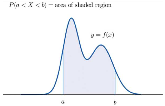
Because of what we know about probabilities, the following is true (and fairly easy to prove):
FACT 4.3.14. Suppose \(f(x)\) is a density function for the continuous RV \(X\) defined on the real interval \([x_{min},x_{max}]\). Then
- For all \(x\) in \([x_{min},x_{max}]\), \(f(x)\ge0\).
- The total area under the curve \(y=f(x)\), above the \(x\)-axis, and between \(x=x_{min}\) and \(x=x_{max}\) is \(1\).
If we want the idea of picking a real number on the interval \([x_{min},x_{max}]\) at random, where at random means that all numbers have the same chance of being picked (along the lines of fair in Definition 4.1.20, the height of the density function must be the same at all \(x\). In other words, the density function \(f(x)\) must be a constant \(c\). In fact, because of the above Fact 4.3.14, that constant must have the value \(\frac1{x_{max}-x_{min}}\). There is a name for this:
DEFINITION 4.3.15. The uniform distribution on \([x_{min},x_{max}]\) is the distribution for the continuous RV whose values are the interval \([x_{min},x_{max}]\) and whose density function is the constant function \(f(x)=\frac1{x_{max}-x_{min}}\).
EXAMPLE 4.3.16. Suppose you take a bus to school every day and because of a chaotic home life (and, let’s face it, you don’t like mornings), you get to the bus stop at a pretty nearly perfectly random time. The bus also doesn’t stick perfectly to its schedule – but it is guaranteed to come at least every \(30\) minutes. What this adds up to is the idea that your waiting time at the bus stop is a uniformly distributed RV on the interval \([0,30]\).
If you wonder one morning how likely it then is that you will wait for less than \(10\) minutes, you can simply compute the area of the rectangle whose base is the interval \([0,10]\) on the \(x\)-axis and whose height is \(\frac1{30}\), which will be \[P(0<X<10)=base \cdot height =10\cdot\frac1{30}=\frac13\ .\] A picture which should clarify this is
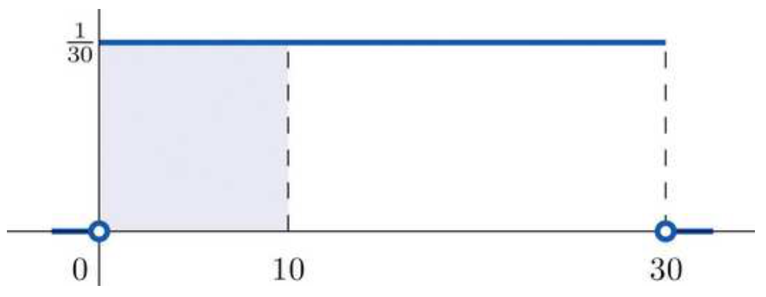
where the area of the shaded region represents the probability of having a waiting time from \(0\) to \(10\) minutes.
One technical thing that can be confusing about continuous RVs and their density functions is the question of whether we should write \(P(a<X<b)\) or \(P(a\le X\le b)\). But if you think about it, we really have three possible events here: \[\begin{aligned} A &= \{\text{outcomes such that } X=a\},\\ M &= \{\text{ outcomes such that $a<X<b$}\},\text{and}\\ B &= \{\text{ outcomes such that $X=b$}\}\ .\end{aligned}\] Since \(X\) always takes on exactly one value for any particular outcome, there is no overlap between these events: they are all disjoint. That means that \[P(A\cup M\cup B) = P(A)+P(M)+P(B) = P(M)\] where the last equality is because, as we said above, the probability of a continuous RV taking on exactly one particular value, as it would in events \(A\) and \(B\), is \(0\). The same would be true if we added merely one endpoint of the interval \((a,b)\). To summarize:
FACT 4.3.17. If \(X\) is a continuous RV with values forming the interval \([x_{min},x_{max}]\) and \(a\) and \(b\) are in this interval, then \[P(a<X<b) = P(a<X\le b) = P(a\le X<b) = P(a\le X\le b)\ .\]
As a consequence of this fact, some authors write probability formulæ about continuous RVs with “\({}<{}\)” and some with “\({}\le{}\)” and it makes no difference.
Let’s do a slightly more interesting example than the uniform distribution:
EXAMPLE 4.3.18. Suppose you repeatedly throw darts at a dartboard. You’re not a machine, so the darts hit in different places every time and you think of this as a repeatable random experiment whose outcomes are the locations of the dart on the board. You’re interested in the probabilities of getting close to the center of the board, so you decide for each experimental outcome (location of a dart you threw) to measure its distance to the center – this will be your RV \(X\).
Being good at this game, you hit near the center more than near the edge and you never completely miss the board, whose radius is \(10cm\)– so \(X\) is more likely to be near \(0\) than near \(10\), and it is never greater than \(10\). What this means is that the RV has values forming the interval \([0,10]\) and the density function, defined on the same interval, should have its maximum value at \(x=0\) and should go down to the value \(0\) when \(x=10\).
You decide to model this situation with the simplest density function you can think of that has the properties we just noticed: a straight line from the highest point of the density function when \(x=0\) down to the point \((10,0)\). The figure that will result will be a triangle, and since the total area must be \(1\) and the base is \(10\) units long, the height must be \(.2\) units. [To get that, we solved the equation \(1=\frac12bh=\frac1210h=5h\) for \(h\).] So the graph must be

and the equation of this linear density function would be \(y=-\frac1{50}x+.2\) [why? – think about the slope and \(y\)-intercept!].
To the extent that you trust this model, you can now calculate the probabilities of events like, for example, “hitting the board within that center bull’s-eye of radius \(1.5cm\),” which probability would be the area of the shaded region in this graph:

The upper-right corner of this shaded region is at \(x\)-coordinate \(1.5\) and is on the line, so its \(y\)-coordinate is \(-\frac1{50}1.5+.2=.17\) . Since the region is a trapezoid, its area is the distance between the two parallel sides times the average of the lengths of the other two sides, giving \[P(0<X<1.5) = 1.5\cdot\frac{.2+.17}2 = .2775\ .\] In other words, the probability of hitting the bull’s-eye, assuming this model of your dart-throwing prowess, is about \(28\)%.
If you don’t remember the formula for the area of a trapezoid, you can do this problem another way: compute the probability of the complementary event, and then take one minus that number. The reason to do this would be that the complementary event corresponds to the shaded region here

which is a triangle! Since we surely do remember the formula for the area of a triangle, we find that \[P(1.5<X<10)=\frac12bh=\frac{1}{2}.17\cdot8.5=.7225\] and therefore \(P(0<X<1.5)=1-P(1.5<X<10)=1-.7225=.2775\). [It’s nice that we got the same number this way, too!]
The Normal Distribution
We’ve seen some examples of continuous RVs, but we have yet to meet the most important one of all.
DEFINITION 4.3.19. The Normal distribution with mean \(\ \mu X\) and standard deviation \(\ \sigma X\) is the continuous RV which takes on all real values and is governed by the probability density function \[\rho(x)=\frac1{\sqrt{2 \sigma X^2\pi}}e^{-\frac{(x- \mu X)^2}{2 \sigma X^2}}\ .\] If \(X\) is a random variable which follows this distribution, then we say that \(X\) is Normally distributed with mean \(\ \mu X\) and standard deviation \(\ \sigma X\) or, in symbols, \(X\) is \(N(\ \mu X, \sigma X)\).
[More technical works also call this the Gaussian distribution, named after the great mathematician Carl Friedrich Gauss. But we will not use that term again in this book after this sentence ends.]
The good news about this complicated formula is that we don’t really have to do anything with it. We will collect some properties of the Normal distribution which have been derived from this formula, but these properties are useful enough, and other tools such as modern calculators and computers which can find specific areas we need under the graph of \(y=\rho(x)\), that we won’t need to work directly with the above formula for \(\rho(x)\) again. It is nice to know that \(N(\mu X, \sigma X)\) does correspond to a specific, known density function, though, isn’t it?
It helps to start with an image of what the Normal distribution looks like. Here is the density function for \(\mu X=17\) and \(\sigma X=3\):
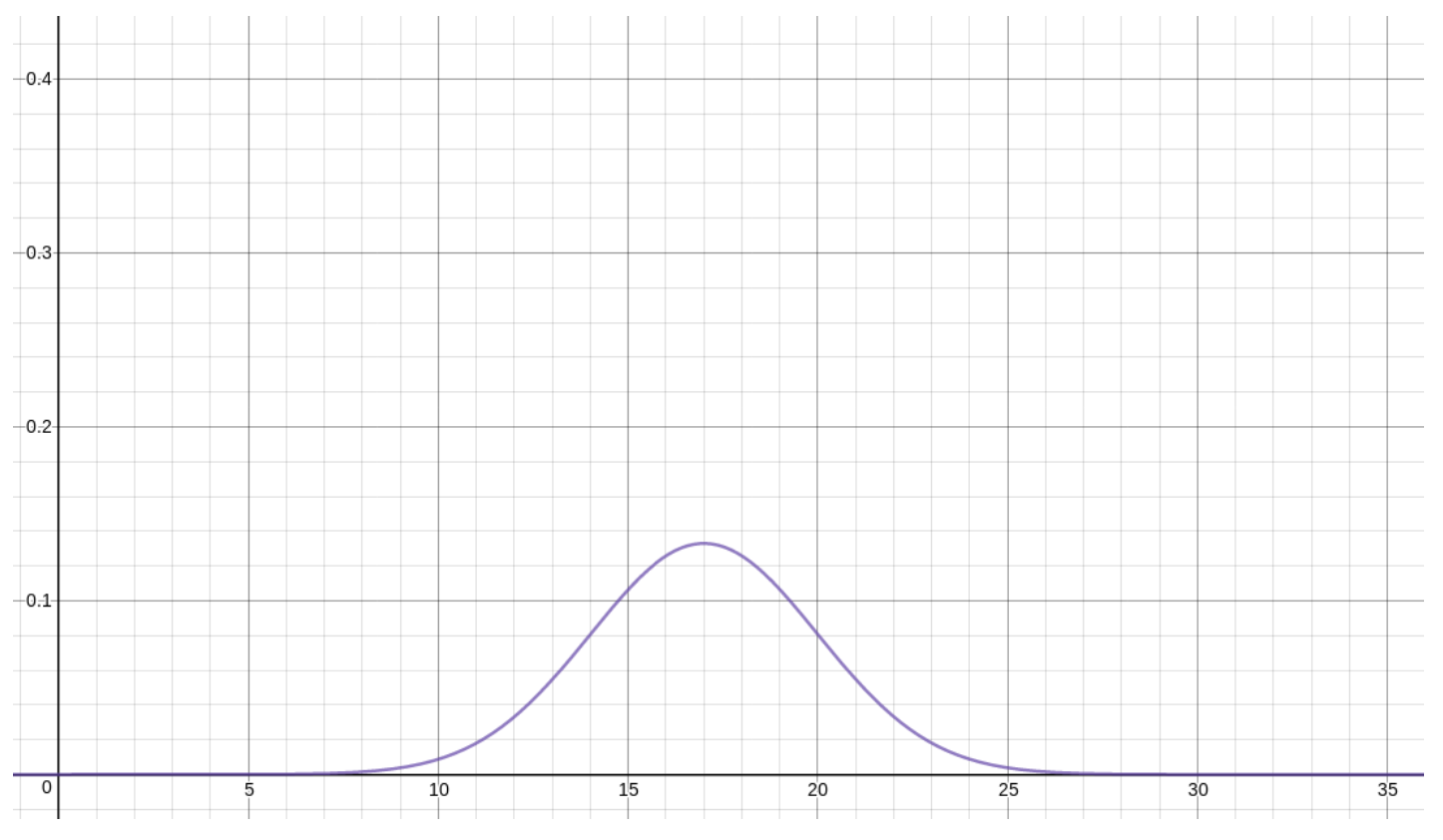
Now let’s collect some of these useful facts about the Normal distributions.
FACT 4.3.20. The density function ρ for the Normal distribution N(μX,σX) is a positive function for all values of x and the total area under the curve y = ρ(x) is 1.
This simply means that ρ is a good candidate for the probability density function for some continuous RV.
FACT 4.3.21. The density function ρ for the Normal distribution N (μX,σX) is unimodal with maximum at x-coordinate μX.
This means that N (μX , σX ) is a possible model for an RV X which tends to have one main, central value, and less often has other values farther away. That center is at the location given by the parameter μX , so wherever we want to put the center of our model for X, we just use that for μX.
FACT 4.3.22. The density function ρ for the Normal distribution N (μX, σX) is symmetric when reflected across the line x = μX.
This means that the amount X misses its center, μX, tends to be about the same when it misses above μX and when it misses below μX. This would correspond to situations were you hit as much to the right as to the left of the center of a dartboard. Or when randomly picked people are as likely to be taller than the average height as they are to be shorter. Or when the time it takes a student to finish a standardized test is as likely to be less than the average as it is to be more than the average. Or in many, many other useful situations.
FACT 4.3.23. The density function ρ for the Normal distribution N(μX,σX) has has tails in both directions which are quite thin, in fact get extremely thin as x → ±∞, but never go all the way to 0.
This means that N(μX,σX) models situations where the amount X deviates from its average has no particular cut-off in the positive or negative direction. So you are throwing darts at a dart board, for example, and there is no way to know how far your dart may hit to the right or left of the center, maybe even way off the board and down the hall – although that may be very unlikely. Or perhaps the time it takes to complete some task is usually a certain amount, but every once and a while it might take much more time, so much more that there is really no natural limit you might know ahead of time.
At the same time, those tails of the Normal distribution are so thin, for values far away from μX , that it can be a good model even for a situation where there is a natural limit to the values of X above or below μX. For example, heights of adult males (in inches) in the United States are fairly well approximated by N(69,2.8), even though heights can never be less than 0 and N (69, 2.8) has an infinitely long tail to the left – because while that tail is non-zero all the way as x → −∞, it is very, very thin.
All of the above Facts are clearly true on the first graph we saw of a Normal distribution density function.
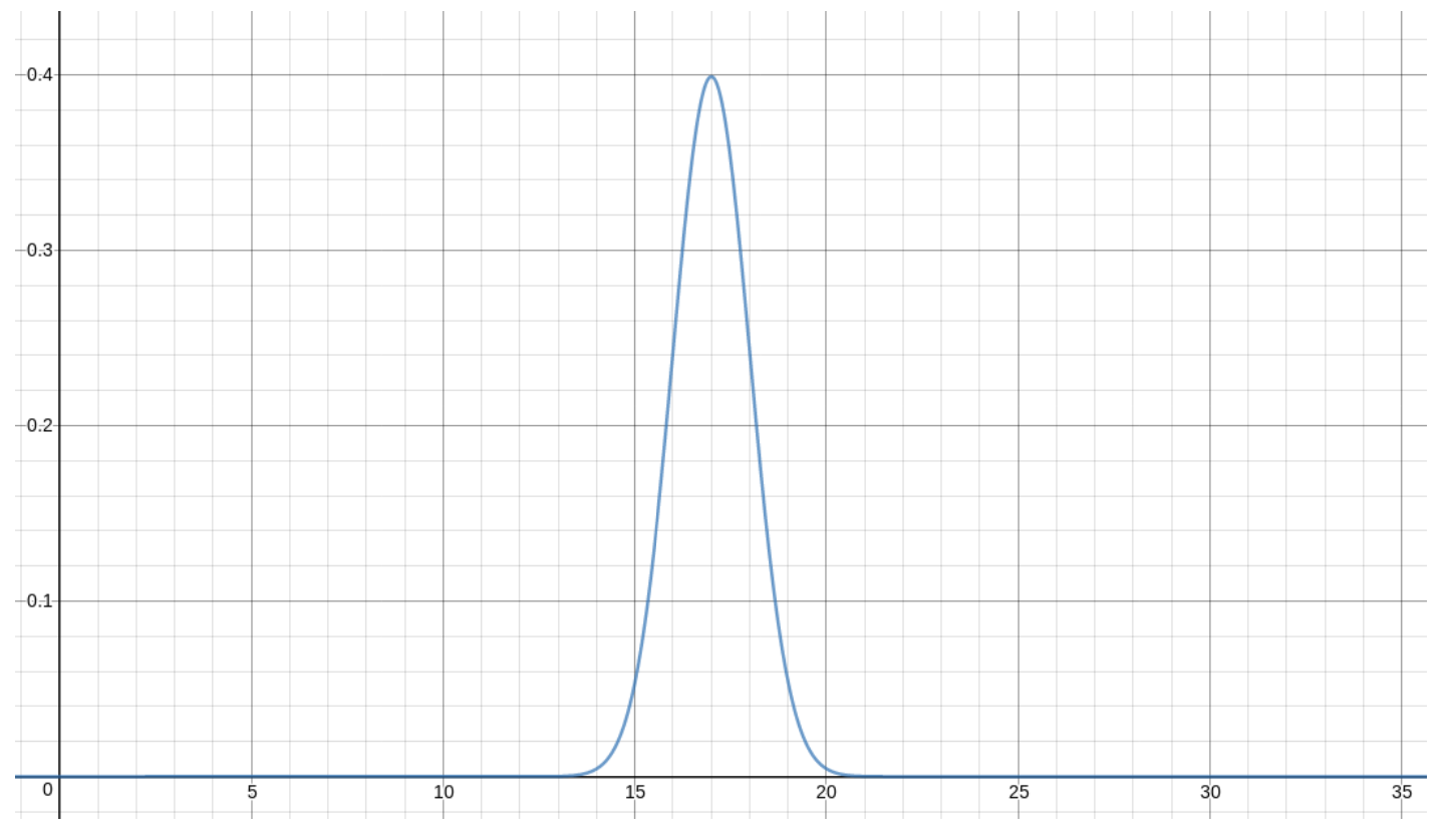
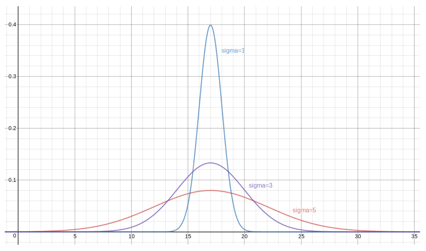
FACT 4.3.24. The graph of the density function ρ for the Normal distribution N(μX,σX) has a taller and narrower peak if σX is smaller, and a lower and wider peak if σX is larger.
This allows the statistician to adjust how much variation there typically is in a normally distributed RV: By making σX small, we are saying that an RV X which is N(μX,σX) is very likely to have values quite close to its center, μX. If we make σX large, however, X is more likely to have values all over the place – still, centered at μX, but more likely to wander farther away.
Let’s make a few versions of the graph we saw for ρ when μX was 17 and σX was 3, but now with different values of σX. First, if σX = 1, we get
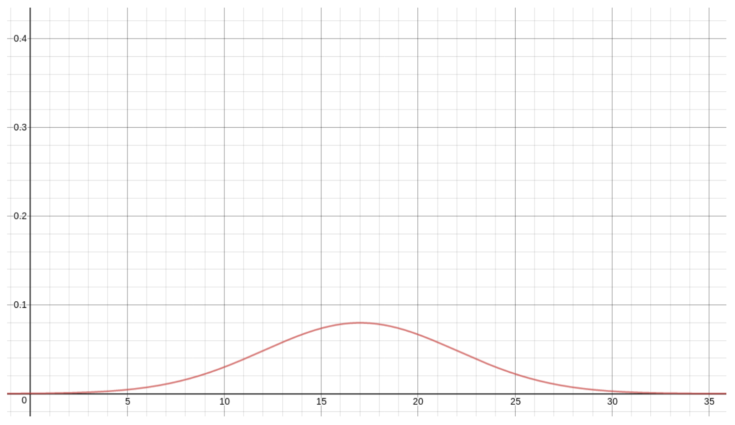
If, instead, σX = 5, then we get
Finally, let’s superimpose all of the above density functions on each other, for one, combined graph:
This variety of Normal distributions (one for each μX and σX ) is a bit bewildering, so traditionally, we concentrate on one particularly nice one.
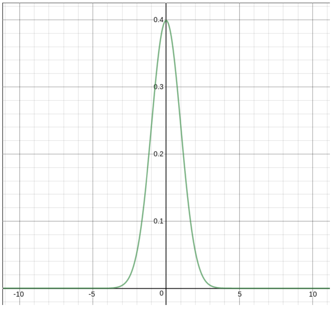
DEFINITION 4.3.25. The Normal distribution with mean μX = 0 and standard deviation σX = 1 is called the standard Normal distribution and an RV [often written with the variable Z ] that is N (0, 1) is described as a standard Normal RV.Here is what the standard Normal probability density function looks like:
Here is what the standard Normal probability density function looks like:
One nice thing about the standard Normal is that all other Normal distributions can be related to the standard.
FACT 4.3.26. If X is N(μX,σX), then Z = (X−μX)/σX is standard Normal.
This has a name.
DEFINITION 4.3.27. The process of replacing a random variable X which is N(μX, σX) with the standard normal RV Z = (X − μX )/σX is called standardizing a Normal RV.
It used to be that standardization was an important step in solving problems with Normal RVs. A problem would be posed with information about some data that was modelled by a Normal RV with given mean μX and standardization σX . Then questions about probabilities for that data could be answered by standardizing the RV and looking up values in a single table of areas under the standard Normal curve.
Today, with electronic tools such as statistical calculators and computers, the standardization step is not really necessary.
EXAMPLE 4.3.28. As we noted above, the heights of adult men in the United States, when measured in inches, give a RV \(X\) which is \(N(69, 2.8)\). What percentage of the population, then, is taller than \(6\) feet?
First of all, the frequentist point of view on probability tells us that what we are interested in is the probability that a randomly chosen adult American male will be taller than 6 feet – that will be the same as the percentage of the population this tall. In other words, we must find the probability that X > 72, since in inches, 6 feet becomes 72. As X is a continuous RV, we must find the area under its density curve, which is the ρ for N (69, 2.8), between 72 and ∞.
That ∞ is a little intimidating, but since the tails of the Normal distribution are very thin, we can stop measuring area when x is some large number and we will have missed only a very tiny amount of area, so we will have a very good approximation. Let’s therefore find the area under ρ from x = 72 up to x = 1000. This can be done in many ways:
- With a wide array of online tools – just search for “online normal probability calculator.” One of these yields the value .142.
- With a TI-8x calculator, by typing
normalcdf(72, 1000, 69, 2.8)
which yields the value .1419884174. The general syntax here is
normalcdf(a, b, μX, σX)
to find P(a < X < b) when X is N(μX,σX). Note you get normalcdf by typing

- Spreadsheets like LibreOffice Calc and Microsoft Excel will compute this by putting the following in a cell
=1-NORM.DIST(72, 69, 2.8, 1)
giving the value 0.1419883859. Here we are using the command
NORM.DIST(b, μX, σX, 1)
which computes the area under the density function for N (μX, σX) from −∞ to b. [The last input of “1” to NORM.DIST just tells it that we want to compute the area under the curve. If we used “0” instead, it would simple tell us the particular value of ρ(b), which is of very direct little use in probability calculations.] Therefore, by doing 1 − NORM.DIST(72,69,2.8,1), we are taking the total area of 1 and subtracting the area to the left of 72, yielding the area to the right, as we wanted.
Therefore, if you want the area between a and b on an N(μX, σX) RV using a spreadsheet, you would put
=NORM.DIST(b, μX, σX, 1) - NORM.DIST(a, μX, σX, 1)
in a cell.
While standardizing a non-standard Normal RV and then looking up values in a table is an old-fashioned method that is tedious and no longer really needed, one old technique still comes in handy some times. It is based on the following:
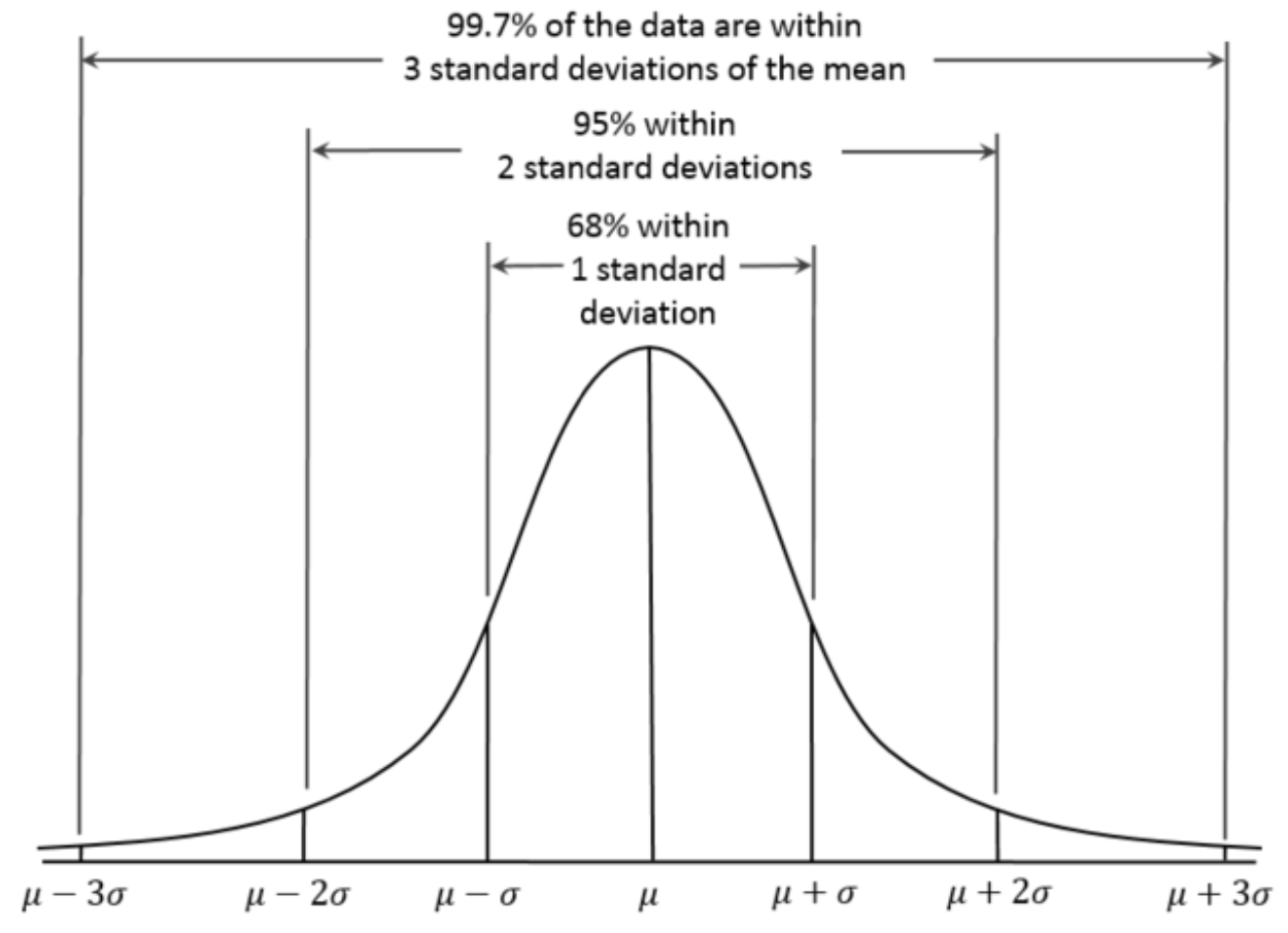
FACT 4.3.29. The 68-95-99.7 Rule: Let X be an N(μX ,σX) RV. Then some special values of the area under the graph of the density curve ρ for X are nice to know:
- The area under the graph of ρ from x=μX −σX to x=μX +σX, also known as P(μX −σX <X<μX +σX), is .68.
- The area under the graph of ρ from x=μX −2σX to x=μX +2σX, also known as P(μX −2σX <X <μX +2σX), is .95.
- The area under the graph of ρ from x=μX −3σX to x=μX +3σX, also known as P(μX −3σX <X <μX +3σX), is .997.
This is also called The Empirical Rule by some authors. Visually3:
3By Dan Kernler - Own work, CC BY-SA 4.0, commons.wikimedia.org/w/index. php?curid=36506025 .
In order to use the 68-95-99.7 Rule in understanding a particular situation, it is helpful to keep an eye out for the numbers that it talks about. Therefore, when looking at a problem, one should notice if the numbers μX +σX, μX −σX, μX +2σX, μX −2σX, μX +3σX, or μX − 3σX are ever mentioned. If so, perhaps this Rule can help.
EXAMPLE 4.3.30. In Example 4.3.28, we needed to compute P(X > 72) where X was known to be N(69,2.8). Is 72 one of the numbers for which we should be looking, to use the Rule? Well, it’s greater than μX = 69, so we could hope that it was μX + σX , μX + 2σX, or μX + 3σX. But values are
μX +σX =69+2.8=71.8,
μX +2σX =69+5.6=74.6,and
μX +3σX =69+8.4=77.4,
none of which is what we need.
Well, it is true that 72 ≈ 71.8, so we could use that fact and accept that we are only getting an approximate answer – an odd choice, given the availability of tools which will give us extremely precise answers, but let’s just go with it for a minute.
Let’s see, the above Rule tells us that
P(66.2<X <71.8)=P(μX −σX <X <μX +σX)=.68.
Now since the total area under any density curve is 1,
P(X <66.2orX >71.8)=1−P(66.2<X <71.8)=1−.68=.32.
Since the event “X < 66.2” is disjoint from the event “X > 71.8” (X only takes on one value at a time, so it cannot be simultaneously less than 66.2 and greater than 71.8), we can use the simple rule for addition of probabilities:
.32=P(X <66.2orX >71.8)=P(X <66.2)+P(X >71.8).
Now, since the density function of the Normal distribution is symmetric around the line x = μX, the two terms on the right in the above equation are equal, which means that
P(X >71.8)=\(\ \frac{1}{2}\) (P(X <66.2)+P(X >71.8))=\(\ \frac{1}{2}\).32=.16.
It might help to visualize the symmetry here as the equality of the two shaded areas in the following graph
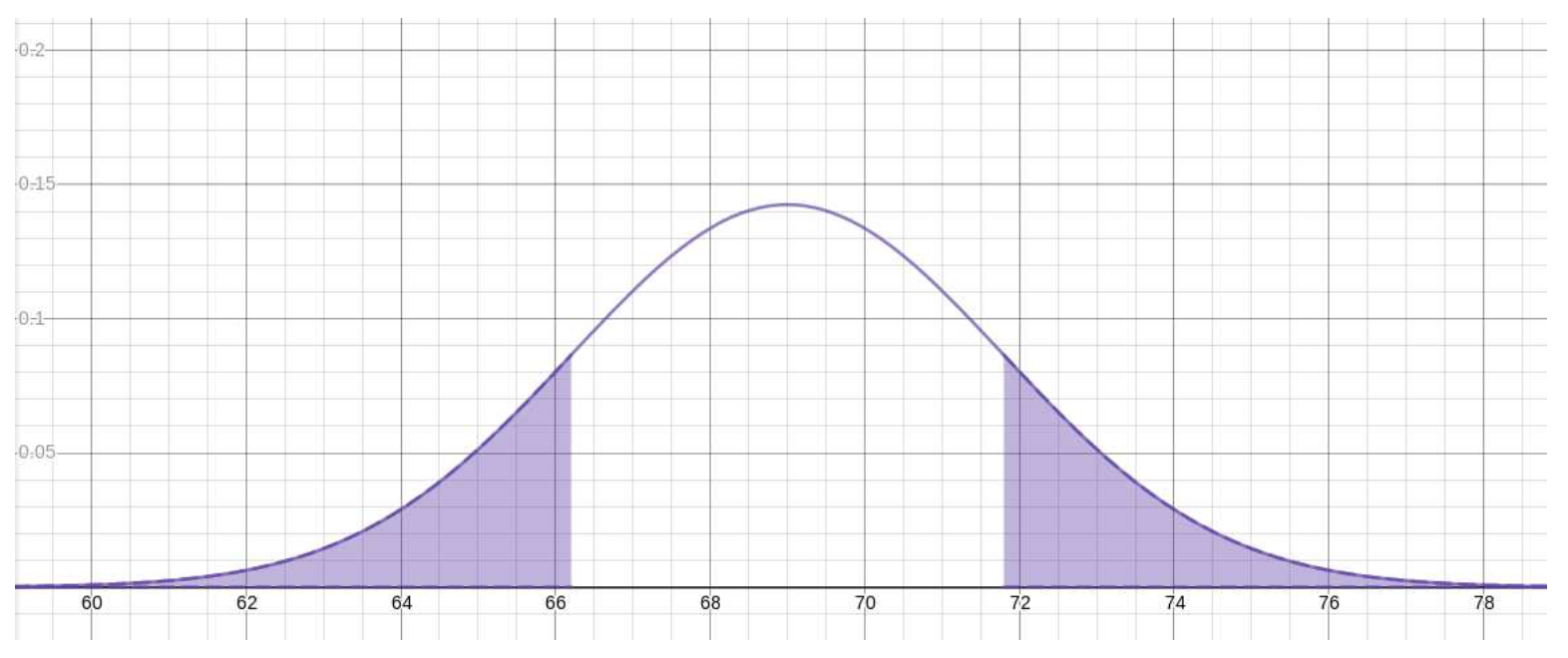
Now, using the fact that 72 ≈ 71.8, we may say that
P (X > 72) ≈ P (X > 71.8) = .16
which, since we know that in fact P (X > 72) = .1419883859, is not a completely terrible approximation.
EXAMPLE 4.3.31. Let’s do one more computation in the context of the heights of adult American males, as in the immediately above Example 4.3.30, but now one in which the 68-95-99.7 Rule gives a more precise answer.
So say we are asked this time what proportion of adult American men are shorter than 63.4 inches. Why that height, in particular? Well, it’s how tall archaeologists have deter- mined King Tut was in life. [No, that’s made up. It’s just a good number for this problem.]
Again, looking through the values μX ± σX, μX ± 2σX, and μX ± 3σX, we notice that
63.4=69−5.6=μX −2σX .
Therefore, to answer what fraction of adult American males are shorter than 63.4 inches amounts to asking what is the value of P (X < μX − 2σX).
What we know about μX ± 2σX is that the probability of X being between those two values is P(μX − 2σX < X < μX + 2σX) = .95. As in the previous Example, the complementary event to “μX − 2σX < X < μX + 2σX,” which will have probability .05, consists of two pieces “X < μX − 2σX” and “X > μX + 2σX,” which have the same area by symmetry. Therefore
\(\begin{aligned} P(X<63.4) &=P\left(X<\mu_{X}-2 \sigma_{X}\right) \\ &=\frac{1}{2}\left[P\left(X<\mu_{X}-2 \sigma_{X}\right)+P\left(X>\mu_{X}+2 \sigma_{X}\right)\right] \\ &=\frac{1}{2} P\left(X<\mu_{X}-2 \sigma_{X} \text { or } X>\mu_{X}+2 \sigma_{X}\right) \text { since they're disjoint } \\ &=\frac{1}{2} P\left(\left(\mu_{X}-2 \sigma_{X}<X<\mu_{X}+2 \sigma_{X}\right)^{c}\right) \\ &=\frac{1}{2}\left[1-P\left(\mu_{X}-2 \sigma_{X}<X<\mu_{X}+2 \sigma_{X}\right)^{c}\right) \quad \\ &=\frac{1}{2}\left[1-P\left(\mu_{X}-2 \sigma_{X}<X<\mu_{X}+2 \sigma_{X}\right)^{c}\right) \quad \text { by prob. for complements } \\ &=\frac{1}{2} \cdot 05 \\ &=.025 \end{aligned}\)
Just the way finding the particular X values μX ± σX, μX ± 2σX, and μX ± 3σX in a particular situation would tell us the 68-95-99.7 Rule might be useful, so also would finding the probability values .68, .95, 99.7, or their complements .32, .05, or .003, – or even half of one of those numbers, using the symmetry.
EXAMPLE 4.3.32. Continuing with the scenario of Example 4.3.30, let us now figure out what is the height above which there will only be .15% of the population.
Notice that .15%, or the proportion .0015, is not one of the numbers in the 68-95-99.7 Rule, nor is it one of their complements – but it is half of one of the complements, being half of .003 . Now, .003 is the complementary probability to .997, which was the probability in the range μX ± 3σX. As we have seen already (twice), the complementary area to that in the region between μX ± 3σX consists of two thin tails which are of equal area, each of these areas being \(\ \frac{1}{2}\)(1 − .997) = .0015 . This all means that the beginning of that upper tail, above which value lies .15% of the population, is the X value μX +3σX =68+3·2.8=77.4.
Therefore .15% of adult American males are taller than 77.4 inches.


