4.1: Definitions for Probability
- Page ID
- 7804
\( \newcommand{\vecs}[1]{\overset { \scriptstyle \rightharpoonup} {\mathbf{#1}} } \)
\( \newcommand{\vecd}[1]{\overset{-\!-\!\rightharpoonup}{\vphantom{a}\smash {#1}}} \)
\( \newcommand{\id}{\mathrm{id}}\) \( \newcommand{\Span}{\mathrm{span}}\)
( \newcommand{\kernel}{\mathrm{null}\,}\) \( \newcommand{\range}{\mathrm{range}\,}\)
\( \newcommand{\RealPart}{\mathrm{Re}}\) \( \newcommand{\ImaginaryPart}{\mathrm{Im}}\)
\( \newcommand{\Argument}{\mathrm{Arg}}\) \( \newcommand{\norm}[1]{\| #1 \|}\)
\( \newcommand{\inner}[2]{\langle #1, #2 \rangle}\)
\( \newcommand{\Span}{\mathrm{span}}\)
\( \newcommand{\id}{\mathrm{id}}\)
\( \newcommand{\Span}{\mathrm{span}}\)
\( \newcommand{\kernel}{\mathrm{null}\,}\)
\( \newcommand{\range}{\mathrm{range}\,}\)
\( \newcommand{\RealPart}{\mathrm{Re}}\)
\( \newcommand{\ImaginaryPart}{\mathrm{Im}}\)
\( \newcommand{\Argument}{\mathrm{Arg}}\)
\( \newcommand{\norm}[1]{\| #1 \|}\)
\( \newcommand{\inner}[2]{\langle #1, #2 \rangle}\)
\( \newcommand{\Span}{\mathrm{span}}\) \( \newcommand{\AA}{\unicode[.8,0]{x212B}}\)
\( \newcommand{\vectorA}[1]{\vec{#1}} % arrow\)
\( \newcommand{\vectorAt}[1]{\vec{\text{#1}}} % arrow\)
\( \newcommand{\vectorB}[1]{\overset { \scriptstyle \rightharpoonup} {\mathbf{#1}} } \)
\( \newcommand{\vectorC}[1]{\textbf{#1}} \)
\( \newcommand{\vectorD}[1]{\overrightarrow{#1}} \)
\( \newcommand{\vectorDt}[1]{\overrightarrow{\text{#1}}} \)
\( \newcommand{\vectE}[1]{\overset{-\!-\!\rightharpoonup}{\vphantom{a}\smash{\mathbf {#1}}}} \)
\( \newcommand{\vecs}[1]{\overset { \scriptstyle \rightharpoonup} {\mathbf{#1}} } \)
\( \newcommand{\vecd}[1]{\overset{-\!-\!\rightharpoonup}{\vphantom{a}\smash {#1}}} \)
\(\newcommand{\avec}{\mathbf a}\) \(\newcommand{\bvec}{\mathbf b}\) \(\newcommand{\cvec}{\mathbf c}\) \(\newcommand{\dvec}{\mathbf d}\) \(\newcommand{\dtil}{\widetilde{\mathbf d}}\) \(\newcommand{\evec}{\mathbf e}\) \(\newcommand{\fvec}{\mathbf f}\) \(\newcommand{\nvec}{\mathbf n}\) \(\newcommand{\pvec}{\mathbf p}\) \(\newcommand{\qvec}{\mathbf q}\) \(\newcommand{\svec}{\mathbf s}\) \(\newcommand{\tvec}{\mathbf t}\) \(\newcommand{\uvec}{\mathbf u}\) \(\newcommand{\vvec}{\mathbf v}\) \(\newcommand{\wvec}{\mathbf w}\) \(\newcommand{\xvec}{\mathbf x}\) \(\newcommand{\yvec}{\mathbf y}\) \(\newcommand{\zvec}{\mathbf z}\) \(\newcommand{\rvec}{\mathbf r}\) \(\newcommand{\mvec}{\mathbf m}\) \(\newcommand{\zerovec}{\mathbf 0}\) \(\newcommand{\onevec}{\mathbf 1}\) \(\newcommand{\real}{\mathbb R}\) \(\newcommand{\twovec}[2]{\left[\begin{array}{r}#1 \\ #2 \end{array}\right]}\) \(\newcommand{\ctwovec}[2]{\left[\begin{array}{c}#1 \\ #2 \end{array}\right]}\) \(\newcommand{\threevec}[3]{\left[\begin{array}{r}#1 \\ #2 \\ #3 \end{array}\right]}\) \(\newcommand{\cthreevec}[3]{\left[\begin{array}{c}#1 \\ #2 \\ #3 \end{array}\right]}\) \(\newcommand{\fourvec}[4]{\left[\begin{array}{r}#1 \\ #2 \\ #3 \\ #4 \end{array}\right]}\) \(\newcommand{\cfourvec}[4]{\left[\begin{array}{c}#1 \\ #2 \\ #3 \\ #4 \end{array}\right]}\) \(\newcommand{\fivevec}[5]{\left[\begin{array}{r}#1 \\ #2 \\ #3 \\ #4 \\ #5 \\ \end{array}\right]}\) \(\newcommand{\cfivevec}[5]{\left[\begin{array}{c}#1 \\ #2 \\ #3 \\ #4 \\ #5 \\ \end{array}\right]}\) \(\newcommand{\mattwo}[4]{\left[\begin{array}{rr}#1 \amp #2 \\ #3 \amp #4 \\ \end{array}\right]}\) \(\newcommand{\laspan}[1]{\text{Span}\{#1\}}\) \(\newcommand{\bcal}{\cal B}\) \(\newcommand{\ccal}{\cal C}\) \(\newcommand{\scal}{\cal S}\) \(\newcommand{\wcal}{\cal W}\) \(\newcommand{\ecal}{\cal E}\) \(\newcommand{\coords}[2]{\left\{#1\right\}_{#2}}\) \(\newcommand{\gray}[1]{\color{gray}{#1}}\) \(\newcommand{\lgray}[1]{\color{lightgray}{#1}}\) \(\newcommand{\rank}{\operatorname{rank}}\) \(\newcommand{\row}{\text{Row}}\) \(\newcommand{\col}{\text{Col}}\) \(\renewcommand{\row}{\text{Row}}\) \(\newcommand{\nul}{\text{Nul}}\) \(\newcommand{\var}{\text{Var}}\) \(\newcommand{\corr}{\text{corr}}\) \(\newcommand{\len}[1]{\left|#1\right|}\) \(\newcommand{\bbar}{\overline{\bvec}}\) \(\newcommand{\bhat}{\widehat{\bvec}}\) \(\newcommand{\bperp}{\bvec^\perp}\) \(\newcommand{\xhat}{\widehat{\xvec}}\) \(\newcommand{\vhat}{\widehat{\vvec}}\) \(\newcommand{\uhat}{\widehat{\uvec}}\) \(\newcommand{\what}{\widehat{\wvec}}\) \(\newcommand{\Sighat}{\widehat{\Sigma}}\) \(\newcommand{\lt}{<}\) \(\newcommand{\gt}{>}\) \(\newcommand{\amp}{&}\) \(\definecolor{fillinmathshade}{gray}{0.9}\)Sample Spaces, Set Operations, and Probability Models
Let’s get right to the definitions.
DEFINITION 4.1.1. Suppose we have a repeatable experiment we want to investigate probabilistically. The things that happen when we do the experiment, the results of running it, are called the [experimental] outcomes. The set of all outcomes is called the sample space of the experiment. We almost always use the symbol \(S\) for this sample space.
EXAMPLE 4.1.2. Suppose the experiment we are doing is “flip a coin.” Then the sample space would be \(S=\{H, T\}\).
EXAMPLE 4.1.3. For the experiment “roll a [normal, six-sided] die,” the sample space would be \(S=\{1, 2, 3, 4, 5, 6\}\).
EXAMPLE 4.1.4. For the experiment “roll two dice,” the sample space would be \[\begin{aligned} S=\{&11, 12, 13, 14, 15, 16,\\ &21, 22, 23, 24, 25, 26\\ &31, 23, 33, 34, 35, 36\\ &41, 42, 43, 44, 45, 46\\ &51, 52, 53, 54, 55, 56\\ &61, 62, 63, 64, 65, 66\\\end{aligned}\] where the notation “\(nm\)” means “\(1^{st}\) roll resulted in an \(n\), \(2^{nd}\) in an \(m\).”
EXAMPLE 4.1.5. Consider the experiment “flip a coin as many times as necessary to see the first Head.” This would have the infinite sample space \[S=\{H, TH, TTH, TTTH, TTTTH, \dots \} \quad .\]
EXAMPLE 4.1.6. Finally, suppose the experiment is “point a Geiger counter at a lump of radioactive material and see how long you have to wait until the next click.” Then the sample space \(S\) is the set of all positive real numbers, because potentially the waiting time could be any positive amount of time.
As mentioned in the chapter introduction, we are more interested in
DEFINITION 4.1.7. Given a repeatable experiment with sample space \(S\), an event is any collection of [some, all, or none of the] outcomes in \(S\); i.e., an event is any subset \(E\) of \(S\), written \(E\subset S\).
There is one special set which is a subset of any other set, and therefore is an event in any sample space.
DEFINITION 4.1.8. The set \(\{\}\) with no elements is called the empty set, for which we use the notation \(\emptyset\).
EXAMPLE 4.1.9. Looking at the sample space \(S=\{H, T\}\) in Example 4.1.2, it’s pretty clear that the following are all the subsets of \(S\): \[\begin{aligned} &\emptyset\\ &\{H\}\\ &\{T\}\\ &S\ [=\{H, T\}]\end{aligned}\]
Two parts of that example are always true: \(\emptyset\) and \(S\) are always subsets of any set \(S\).
Since we are going to be working a lot with events, which are subsets of a larger set, the sample space, it is nice to have a few basic terms from set theory:
DEFINITION 4.1.10. Given a subset E ⊂ S of a larger set S, the complement of E, is the set Ec = {all the elements of S which are not in E}.
If we describe an event \(E\) in words as all outcomes satisfies some property \(X\), the complementary event, consisting of all the outcomes not in \(E\), can be described as all outcomes which don’t satisfy \(X\). In other words, we often describe the event \(E^c\) as the event “not \(E\).”
DEFINITION 4.1.11. Given two sets \(A\) and \(B\), their union is the set \[A\cup B = \{\text{all elements which are in A or B [or both]}\}\ .\]
Now if event \(A\) is those outcomes having property \(X\) and \(B\) is those with property \(Y\), the event \(A\cup B\), with all outcomes in \(A\) together with all outcomes in \(B\) can be described as all outcomes satisfying \(X\) or \(Y\), thus we sometimes pronounce the event “\(A\cup B\)” as “\(A\) or \(B\).”
DEFINITION 4.1.12. Given two sets \(A\) and \(B\), their intersection is the set \[A\cap B = \{\text{all elements which are in both A and B}\}\ .\]
If, as before, event \(A\) consists of those outcomes having property \(X\) and \(B\) is those with property \(Y\), the event \(A\cap B\) will consist of those outcomes which satisfy both \(X\) and \(Y\). In other words, “\(A\cap B\)” can be described as “\(A\) and \(B\).”
Putting together the idea of intersection with the idea of that special subset \(\emptyset\) of any set, we get the
DEFINITION 4.1.13. Two sets \(A\) and \(B\) are called disjoint if \(A\cap B=\emptyset\). In other words, sets are disjoint if they have nothing in common.
A exact synonym for disjoint that some authors prefer is mutually exclusive. We will use both terms interchangeably in this book.
Now we are ready for the basic structure of probability.
DEFINITION 4.1.14. Given a sample space \(S\), a probability model on \(S\) is a choice of a real number \(P(E)\) for every event \(E\subset S\) which satisfies
- For all events \(E\), \(0\le P(E)\le 1\).
- \(P(\emptyset)=1\) and \(P(S)=1\).
- For all events \(E\), \(P(E^c)=1-P(E)\).
- If \(A\) and \(B\) are any two disjoint events, then \(P(A\cup B)=P(A)+P(B)\). [This is called the addition rule for disjoint events.]
Venn Diagrams
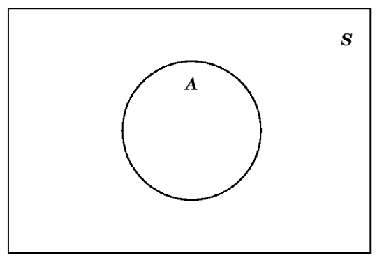
Venn diagrams are a simple way to display subsets of a fixed set and to show the relationships between these subsets and even the results of various set operations (like complement, union, and intersection) on them. The primary use we will make of Venn diagrams is for events in a certain sample space, so we will use that terminology [even though the technique has much wider application].
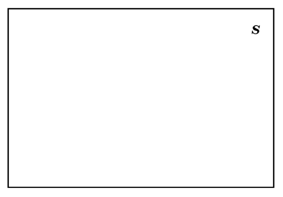
To make a Venn Diagram, always start out by making a rectangle to represent the whole sample space:
Within that rectangle, we make circles, ovals, or just blobs, to indicate that portion of the sample space which is some event \(E\):
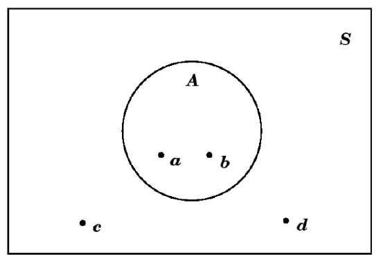
Sometimes, if the outcomes in the sample space \(S\) and in the event \(A\) might be indicated in the different parts of the Venn diagram. So, if \(S=\{a, b, c, d\}\) and \(A=\{a, b\}\subset S\), we might draw this as
The complement \(E^c\) of an event \(E\) is easy to show on a Venn diagram, since it is simply everything which is not in \(E\):
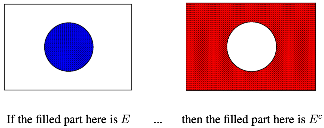
This can actually be helpful in figuring out what must be in \(E^c\). In the example above with \(S=\{a, b, c, d\}\) and \(A=\{a, b\}\subset S\), by looking at what is in the shaded exterior part for our picture of \(E^c\), we can see that for that \(A\), we would get \(A^c=\{c, d\}\).
Moving now to set operations that work with two events, suppose we want to make a Venn diagram with events \(A\) and \(B\). If we know these events are disjoint, then we would make the diagram as follows:
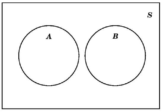
while if they are known not to be disjoint, we would use instead this diagram:
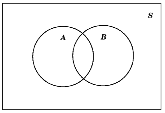
For example, it \(S=\{a, b, c, d\}\), \(A=\{a, b\}\), and \(B=\{b, c\}\), we would have
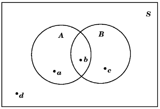
When in doubt, it is probably best to use the version with overlap, which then could simply not have any points in it (or could have zero probability, when we get to that, below).
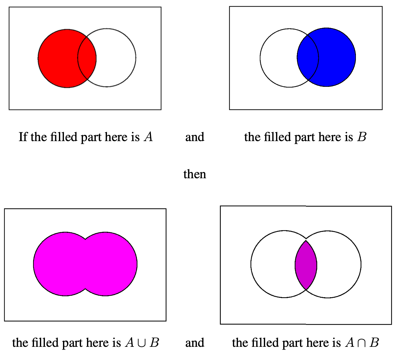
Venn diagrams are very good at showing unions, and intersection:
Another nice thing to do with Venn diagrams is to use them as a visual aid for probability computations. The basic idea is to make a diagram showing the various events sitting inside the usual rectangle, which stands for the sample space, and to put numbers in various parts of the diagram showing the probabilities of those events, or of the results of operations (unions, intersection, and complement) on those events.
For example, if we are told that an event \(A\) has probability \(P(A)=.4\), then we can immediately fill in the \(.4\) as follows:
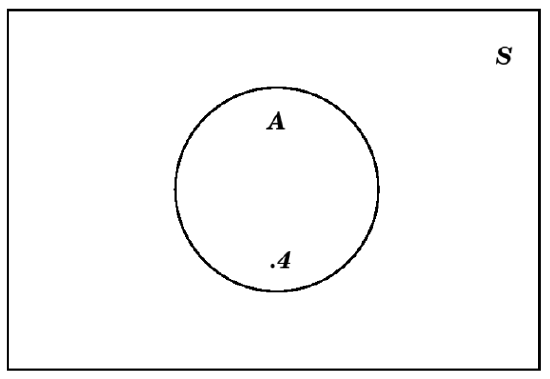
But we can also put a number in the exterior of that circle which represents \(A\), taking advantage of the fact that that exterior is \(A^c\) and the rule for probabilities of complements (point (3) in Definition 4.1.14) to conclude that the appropriate number is \(1-.4=.6\):
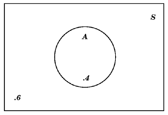
We recommend that, in a Venn diagram showing probability values, you always put a number in the region exterior to all of the events [but inside the rectangle indicating the sample space, of course].
Complicating a little this process of putting probability numbers in the regions of a Venn diagram is the situation where we are giving for both an event and a subsetsubset, \(\subset\) of that event. This most often happens when we are told probabilities both of some events and of their intersection(s). Here is an example:
EXAMPLE 4.1.15. Suppose we are told that we have two events \(A\) and \(B\) in the sample space \(S\), which satisfy \(P(A)=.4\), \(P(B)=.5\), and \(P(A\cap B)=.1\). First of all, we know that \(A\) and \(B\) are not disjoint, since if they were disjoint, that would mean (by definition) that \(A\cap B=\emptyset\), and since \(P(\emptyset)=0\) but \(P(A\cap B)\neq 0\), that is not possible. So we draw a Venn diagram that we’ve see before:
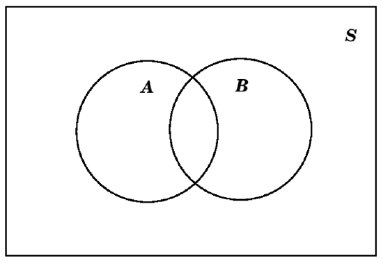
However, it would be unwise simply to write those given numbers \(.4\), \(.5\), and \(.1\) into the three central regions of this diagram. The reason is that the number \(.1\) is the probability of \(A\cap B\), which is a part of \(A\) already, so if we simply write \(.4\) in the rest of \(A\), we would be counting that \(.1\) for the \(A\cap B\) twice. Therefore, before we write a number in the rest of \(A\), outside of \(A\cap B\), we have to subtract the \(.1\) for \(P(A\cap B)\). That means that the number which goes in the rest of \(A\) should be \(.4-.1=.3\). A similar reasoning tells us that the number in the part of \(B\) outside of \(A\cap B\), should be \(.5-.1=.4\). That means the Venn diagram with all probabilities written in would be:
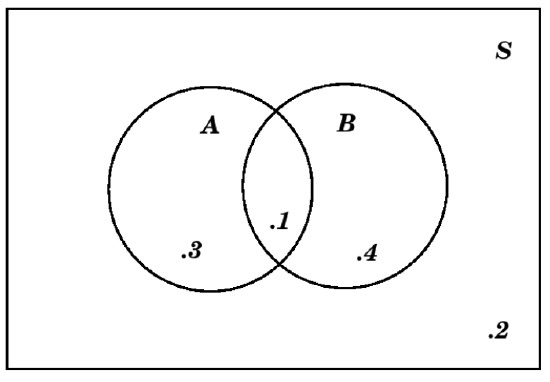
The approach in the above example is our second important recommendation for who to put numbers in a Venn diagram showing probability values: always put a number in each region which corresponds to the probability of that smallest connected region containing the number, not any larger region.
One last point we should make, using the same argument as in the above example. Suppose we have events \(A\) and \(B\) in a sample space \(S\) (again). Suppose we are not sure if \(A\) and \(B\) are disjoint, so we cannot use the addition rule for disjoint events to compute \(P(A\cup B)\). But notice that the events \(A\) and \(A^c\) are disjoint, so that \(A\cap B\) and \(A^c\cap B\) are also disjoint and \[A = A\cap S = A\cap\left(B\cup B^c\right) = \left(A\cap B\right)\cup\left(A\cap B^c\right)\] is a decomposition of the event \(A\) into the two disjoint events \(A\cap B\) and \(A^c\cap B\). From the addition rule for disjoint events, this means that \[P(A)=P(A\cap B)+P(A\cap B^c)\ .\]
Similar reasoning tells us both that \[P(B)=P(A\cap B)+P(A^c\cap B)\] and that \[A\cup B=\left(A\cap B^c\right)\cup\left(A\cap B\right)\cup\left(A^c\cap B\right)\] is a decomposition of \(A\cup B\) into disjoint pieces, so that \[P(A\cup B)=P(A\cap B^c)+P(A\cap B)+P(A^c\cap B)\ .\] Combining all of these equations, we conclude that \[\begin{aligned} P(A)+P(B)-P(A\cap B) &=P(A\cap B)+P(A\cap B^c)+P(A\cap B)+P(A^c\cap B)-P(A\cap B)\\ &= P(A\cap B^c)+P(A\cap B)+P(A^c\cap B) + P(A\cap B)-P(A\cap B)\\ &= P(A\cap B^c)+P(A\cap B)+P(A^c\cap B)\\ &= P(A\cup B) \ .\end{aligned}\] This is important enough to state as a
FACT 4.1.16. The Addition Rule for General Events If \(A\) and \(B\) are events in a sample space \(S\) then we have the addition rule for their probabilities \[P(A\cup B) = P(A) + P(B) - P(A\cap B)\ .\] This rule is true whether or not \(A\) and \(B\) are disjoint.
Finite Probability Models
Here is a nice situation in which we can easily calculate a lot of probabilities fairly easily: if the sample space \(S\) of some experiment is finite.
So let’s suppose the sample space consists of just the outcomes \(S=\{o_1, o_2, \dots, o_n\}\). For each of the outcomes, we can compute the probability: \[\begin{aligned} p_1 =& P(\{o_1\})\\ p_2 =& P(\{o_2\})\\ &\vdots\\ p_n =& P(\{o_n\})\\\end{aligned}\] Let’s think about what the rules for probability models tell us about these numbers \(p_1, p_2, \dots, p_n\). First of all, since they are each the probability of an event, we see that \[\begin{aligned} 0\le &p_1\le 1\\ 0\le &p_2\le 1\\ &\ \vdots\\ 0\le &p_n\le 1\end{aligned}\] Furthermore, since \(S=\{o_1, o_2, \dots, o_n\}=\{o_1\}\cup\{o_2\}\cup \dots \cup\{o_n\}\) and all of the events \(\{o_1\}, \{o_2\}, \dots, \{o_n\}\) are disjoint, by the addition rule for disjoint events we have \[\begin{aligned} 1=P(S)&=P(\{o_1, o_2, \dots, o_n\})\\ &=P(\{o_1\}\cup\{o_2\}\cup \dots \cup\{o_n\})\\ &=P(\{o_1\})+P(\{o_2\})+ \dots +P(\{o_n\})\\ &=p_1+p_2+ \dots +p_n\ .\end{aligned}\]
The final thing to notice about this situation of a finite sample space is that if \(E\subset S\) is any event, then \(E\) will be just a collection of some of the outcomes from \(\{o_1, o_2, \dots, o_n\}\) (maybe none, maybe all, maybe an intermediate number). Since, again, the events like \(\{o_1\}\) and \(\{o_2\}\) and so on are disjoint, we can compute \[\begin{aligned} P(E) &= P(\{\text{the outcomes $o_j$ which make up $E$}\})\\ &= \sum \{\text{the $p_j$'s for the outcomes in $E$}\}\ .\end{aligned}\]
In other words
FACT 4.1.17. A probability model on a sample space \(S\) with a finite number, \(n\), of outcomes, is nothing other than a choice of real numbers \(p_1, p_2, \dots, p_n\), all in the range from \(0\) to \(1\) and satisfying \(p_1+p_2+ \dots +p_n=1\). For such a choice of numbers, we can compute the probability of any event \(E\subset S\) as \[P(E) = \sum \{\text{the p_j's corresponding to the outcomes o_j which make up E}\}\ .\]
EXAMPLE 4.1.18. For the coin flip of Example 4.1.2, there are only the two outcomes \(H\) and \(T\) for which we need to pick two probabilities, call them \(p\) and \(q\). In fact, since the total must be \(1\), we know that \(p+q=1\) or, in other words, \(q=1-p\). The the probabilities for all events (which we listed in Example 4.1.9) are \[\begin{aligned} P(\emptyset) &= 0\\ P(\{H\}) &= p\\ P(\{T\}) &= q = 1-p\\ P(\{H,T\}) &= p + q = 1\end{aligned}\]
What we’ve described here is, potentially, a biased coin, since we are not assuming that \(p=q\) – the probabilities of getting a head and a tail are not assumed to be the same. The alternative is to assume that we have a fair coin, meaning that \(p=q\). Note that in such a case, since \(p+q=1\), we have \(2p=1\) and so \(p=1/2\). That is, the probability of a head (and, likewise, the probability of a tail) in a single throw of a fair coin is \(1/2\).
EXAMPLE 4.1.19. As in the previous example, we can consider the die of Example 4.1.3 to a fair die, meaning that the individual face probabilities are all the same. Since they must also total to \(1\) (as we saw for all finite probability models), it follows that \[p_1 = p_2 = p_3 = p_4 = p_5 = p_6 = 1/6 .\] We can then use this basic information and the formula (for \(P(E)\)) in Fact 4.1.17 to compute the probability of any event of interest, such as \[P(\text{``roll was even''}) = P(\{2, 4, 6\}) = \frac16 + \frac16 + \frac16 = \frac36 = \frac12\ .\]
We should immortalize these last two examples with a
[def:fair] When we are talking about dice, coins, individuals for some task, or another small, practical, finite experiment, we use the term fair to indicate that the probabilities of all individual outcomes are equal (and therefore all equal to the the number \(1/n\), where \(n\) is the number of outcomes in the sample space). A more technical term for the same idea is equiprobable, while a more casual term which is often used for this in very informal settings is “at random” (such as “pick a card at random from this deck” or “pick a random patient from the study group to give the new treatment to...”).
EXAMPLE 4.1.21. Suppose we look at the experiment of Example 4.1.4 and add the information that the two dice we are rolling are fair. This actually isn’t quite enough to figure out the probabilities, since we also have to assure that the fair rolling of the first die doesn’t in any way affect the rolling of the second die. This is technically the requirement that the two rolls be independent, but since we won’t investigate that carefully until §2, below, let us instead here simply say that we assume the two rolls are fair and are in fact completely uninfluenced by anything around them in the world including each other.
What this means is that, in the long run, we would expect the first die to show a \(1\) roughly \({\frac16}^{th}\) of the time, and in the very long run, the second die would show a \(1\) roughly \({\frac16}^{th}\) of those times. This means that the outcome of the “roll two dice” experiment should be \(11\) with probability \(\frac{1}{36}\) – and the same reasoning would show that all of the outcomes have that probability. In other words, this is an equiprobable sample space with \(36\) outcomes each having probability \(\frac{1}{36}\). Which in turn enables us to compute any probability we might like, such as \[\begin{aligned} P(\text{``sum of the two rolls is $4$''}) &= P(\{13, 22, 31\})\\ &= \frac{1}{36} + \frac{1}{36} + \frac{1}{36}\\ &= \frac{3}{36}\\ &= \frac{1}{12}\ .\end{aligned}\]


