
2.5: The Empirical Rule and Chebyshev's Theorem
- Page ID
- 559
\( \newcommand{\vecs}[1]{\overset { \scriptstyle \rightharpoonup} {\mathbf{#1}} } \)
\( \newcommand{\vecd}[1]{\overset{-\!-\!\rightharpoonup}{\vphantom{a}\smash {#1}}} \)
\( \newcommand{\dsum}{\displaystyle\sum\limits} \)
\( \newcommand{\dint}{\displaystyle\int\limits} \)
\( \newcommand{\dlim}{\displaystyle\lim\limits} \)
\( \newcommand{\id}{\mathrm{id}}\) \( \newcommand{\Span}{\mathrm{span}}\)
( \newcommand{\kernel}{\mathrm{null}\,}\) \( \newcommand{\range}{\mathrm{range}\,}\)
\( \newcommand{\RealPart}{\mathrm{Re}}\) \( \newcommand{\ImaginaryPart}{\mathrm{Im}}\)
\( \newcommand{\Argument}{\mathrm{Arg}}\) \( \newcommand{\norm}[1]{\| #1 \|}\)
\( \newcommand{\inner}[2]{\langle #1, #2 \rangle}\)
\( \newcommand{\Span}{\mathrm{span}}\)
\( \newcommand{\id}{\mathrm{id}}\)
\( \newcommand{\Span}{\mathrm{span}}\)
\( \newcommand{\kernel}{\mathrm{null}\,}\)
\( \newcommand{\range}{\mathrm{range}\,}\)
\( \newcommand{\RealPart}{\mathrm{Re}}\)
\( \newcommand{\ImaginaryPart}{\mathrm{Im}}\)
\( \newcommand{\Argument}{\mathrm{Arg}}\)
\( \newcommand{\norm}[1]{\| #1 \|}\)
\( \newcommand{\inner}[2]{\langle #1, #2 \rangle}\)
\( \newcommand{\Span}{\mathrm{span}}\) \( \newcommand{\AA}{\unicode[.8,0]{x212B}}\)
\( \newcommand{\vectorA}[1]{\vec{#1}} % arrow\)
\( \newcommand{\vectorAt}[1]{\vec{\text{#1}}} % arrow\)
\( \newcommand{\vectorB}[1]{\overset { \scriptstyle \rightharpoonup} {\mathbf{#1}} } \)
\( \newcommand{\vectorC}[1]{\textbf{#1}} \)
\( \newcommand{\vectorD}[1]{\overrightarrow{#1}} \)
\( \newcommand{\vectorDt}[1]{\overrightarrow{\text{#1}}} \)
\( \newcommand{\vectE}[1]{\overset{-\!-\!\rightharpoonup}{\vphantom{a}\smash{\mathbf {#1}}}} \)
\( \newcommand{\vecs}[1]{\overset { \scriptstyle \rightharpoonup} {\mathbf{#1}} } \)
\(\newcommand{\longvect}{\overrightarrow}\)
\( \newcommand{\vecd}[1]{\overset{-\!-\!\rightharpoonup}{\vphantom{a}\smash {#1}}} \)
\(\newcommand{\avec}{\mathbf a}\) \(\newcommand{\bvec}{\mathbf b}\) \(\newcommand{\cvec}{\mathbf c}\) \(\newcommand{\dvec}{\mathbf d}\) \(\newcommand{\dtil}{\widetilde{\mathbf d}}\) \(\newcommand{\evec}{\mathbf e}\) \(\newcommand{\fvec}{\mathbf f}\) \(\newcommand{\nvec}{\mathbf n}\) \(\newcommand{\pvec}{\mathbf p}\) \(\newcommand{\qvec}{\mathbf q}\) \(\newcommand{\svec}{\mathbf s}\) \(\newcommand{\tvec}{\mathbf t}\) \(\newcommand{\uvec}{\mathbf u}\) \(\newcommand{\vvec}{\mathbf v}\) \(\newcommand{\wvec}{\mathbf w}\) \(\newcommand{\xvec}{\mathbf x}\) \(\newcommand{\yvec}{\mathbf y}\) \(\newcommand{\zvec}{\mathbf z}\) \(\newcommand{\rvec}{\mathbf r}\) \(\newcommand{\mvec}{\mathbf m}\) \(\newcommand{\zerovec}{\mathbf 0}\) \(\newcommand{\onevec}{\mathbf 1}\) \(\newcommand{\real}{\mathbb R}\) \(\newcommand{\twovec}[2]{\left[\begin{array}{r}#1 \\ #2 \end{array}\right]}\) \(\newcommand{\ctwovec}[2]{\left[\begin{array}{c}#1 \\ #2 \end{array}\right]}\) \(\newcommand{\threevec}[3]{\left[\begin{array}{r}#1 \\ #2 \\ #3 \end{array}\right]}\) \(\newcommand{\cthreevec}[3]{\left[\begin{array}{c}#1 \\ #2 \\ #3 \end{array}\right]}\) \(\newcommand{\fourvec}[4]{\left[\begin{array}{r}#1 \\ #2 \\ #3 \\ #4 \end{array}\right]}\) \(\newcommand{\cfourvec}[4]{\left[\begin{array}{c}#1 \\ #2 \\ #3 \\ #4 \end{array}\right]}\) \(\newcommand{\fivevec}[5]{\left[\begin{array}{r}#1 \\ #2 \\ #3 \\ #4 \\ #5 \\ \end{array}\right]}\) \(\newcommand{\cfivevec}[5]{\left[\begin{array}{c}#1 \\ #2 \\ #3 \\ #4 \\ #5 \\ \end{array}\right]}\) \(\newcommand{\mattwo}[4]{\left[\begin{array}{rr}#1 \amp #2 \\ #3 \amp #4 \\ \end{array}\right]}\) \(\newcommand{\laspan}[1]{\text{Span}\{#1\}}\) \(\newcommand{\bcal}{\cal B}\) \(\newcommand{\ccal}{\cal C}\) \(\newcommand{\scal}{\cal S}\) \(\newcommand{\wcal}{\cal W}\) \(\newcommand{\ecal}{\cal E}\) \(\newcommand{\coords}[2]{\left\{#1\right\}_{#2}}\) \(\newcommand{\gray}[1]{\color{gray}{#1}}\) \(\newcommand{\lgray}[1]{\color{lightgray}{#1}}\) \(\newcommand{\rank}{\operatorname{rank}}\) \(\newcommand{\row}{\text{Row}}\) \(\newcommand{\col}{\text{Col}}\) \(\renewcommand{\row}{\text{Row}}\) \(\newcommand{\nul}{\text{Nul}}\) \(\newcommand{\var}{\text{Var}}\) \(\newcommand{\corr}{\text{corr}}\) \(\newcommand{\len}[1]{\left|#1\right|}\) \(\newcommand{\bbar}{\overline{\bvec}}\) \(\newcommand{\bhat}{\widehat{\bvec}}\) \(\newcommand{\bperp}{\bvec^\perp}\) \(\newcommand{\xhat}{\widehat{\xvec}}\) \(\newcommand{\vhat}{\widehat{\vvec}}\) \(\newcommand{\uhat}{\widehat{\uvec}}\) \(\newcommand{\what}{\widehat{\wvec}}\) \(\newcommand{\Sighat}{\widehat{\Sigma}}\) \(\newcommand{\lt}{<}\) \(\newcommand{\gt}{>}\) \(\newcommand{\amp}{&}\) \(\definecolor{fillinmathshade}{gray}{0.9}\)- To learn what the value of the standard deviation of a data set implies about how the data scatter away from the mean as described by the Empirical Rule and Chebyshev’s Theorem.
- To use the Empirical Rule and Chebyshev’s Theorem to draw conclusions about a data set.
You probably have a good intuitive grasp of what the average of a data set says about that data set. In this section we begin to learn what the standard deviation has to tell us about the nature of the data set.
The Empirical Rule
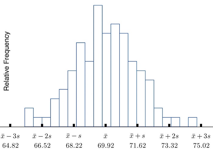
We start by examining a specific set of data. Table \(\PageIndex{1}\) shows the heights in inches of \(100\) randomly selected adult men. A relative frequency histogram for the data is shown in Figure \(\PageIndex{1}\). The mean and standard deviation of the data are, rounded to two decimal places, \(\bar{x}=69.92\) and \(\sigma = 1.70\).
| 68.7 | 72.3 | 71.3 | 72.5 | 70.6 | 68.2 | 70.1 | 68.4 | 68.6 | 70.6 |
| 73.7 | 70.5 | 71.0 | 70.9 | 69.3 | 69.4 | 69.7 | 69.1 | 71.5 | 68.6 |
| 70.9 | 70.0 | 70.4 | 68.9 | 69.4 | 69.4 | 69.2 | 70.7 | 70.5 | 69.9 |
| 69.8 | 69.8 | 68.6 | 69.5 | 71.6 | 66.2 | 72.4 | 70.7 | 67.7 | 69.1 |
| 68.8 | 69.3 | 68.9 | 74.8 | 68.0 | 71.2 | 68.3 | 70.2 | 71.9 | 70.4 |
| 71.9 | 72.2 | 70.0 | 68.7 | 67.9 | 71.1 | 69.0 | 70.8 | 67.3 | 71.8 |
| 70.3 | 68.8 | 67.2 | 73.0 | 70.4 | 67.8 | 70.0 | 69.5 | 70.1 | 72.0 |
| 72.2 | 67.6 | 67.0 | 70.3 | 71.2 | 65.6 | 68.1 | 70.8 | 71.4 | 70.2 |
| 70.1 | 67.5 | 71.3 | 71.5 | 71.0 | 69.1 | 69.5 | 71.1 | 66.8 | 71.8 |
| 69.6 | 72.7 | 72.8 | 69.6 | 65.9 | 68.0 | 69.7 | 68.7 | 69.8 | 69.7 |
If we go through the data and count the number of observations that are within one standard deviation of the mean, that is, that are between \(69.92-1.70=68.22\) and \(69.92+1.70=71.62\) inches, there are \(69\) of them. If we count the number of observations that are within two standard deviations of the mean, that is, that are between \(69.92-2(1.70)=66.52\) and \(69.92+2(1.70)=73.32\) inches, there are \(95\) of them. All of the measurements are within three standard deviations of the mean, that is, between \(69.92-3(1.70)=64.822\) and \(69.92+3(1.70)=75.02\) inches. These tallies are not coincidences, but are in agreement with the following result that has been found to be widely applicable.
The Empirical Rule
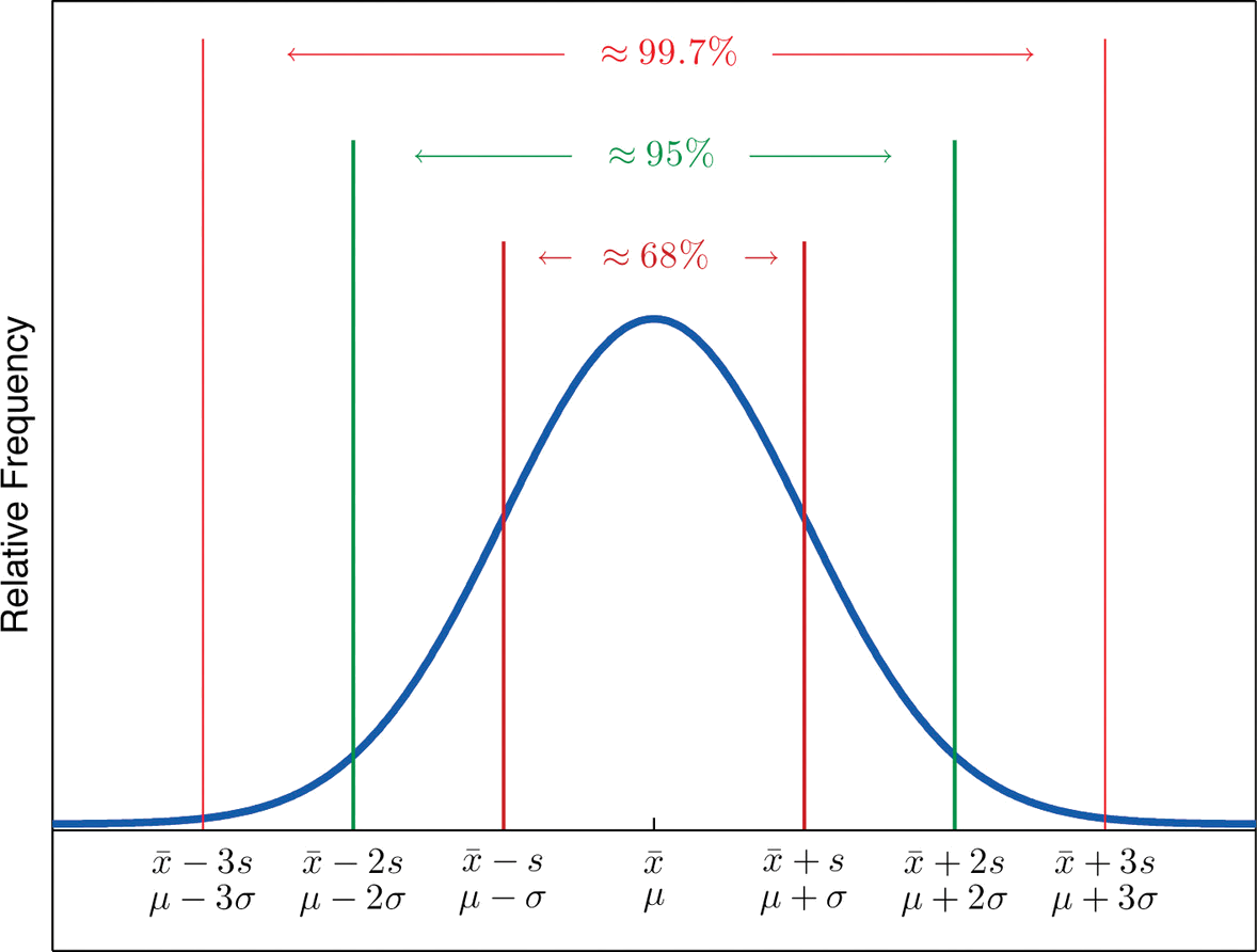
Approximately \(68\%\) of the data lie within one standard deviation of the mean, that is, in the interval with endpoints \(\bar{x}\pm s\) for samples and with endpoints \(\mu \pm \sigma\) for populations; if a data set has an approximately bell-shaped relative frequency histogram, then (Figure \(\PageIndex{2}\))
- approximately \(95\%\) of the data lie within two standard deviations of the mean, that is, in the interval with endpoints \(\bar{x}\pm 2s\) for samples and with endpoints \(\mu \pm 2\sigma\) for populations; and
- approximately \(99.7\%\) of the data lies within three standard deviations of the mean, that is, in the interval with endpoints \(\bar{x}\pm 3s\) for samples and with endpoints \(\mu \pm 3\sigma\) for populations.

Two key points in regard to the Empirical Rule are that the data distribution must be approximately bell-shaped and that the percentages are only approximately true. The Empirical Rule does not apply to data sets with severely asymmetric distributions, and the actual percentage of observations in any of the intervals specified by the rule could be either greater or less than those given in the rule. We see this with the example of the heights of the men: the Empirical Rule suggested 68 observations between \(68.22\) and \(71.62\) inches, but we counted \(69\).
Heights of \(18\)-year-old males have a bell-shaped distribution with mean \(69.6\) inches and standard deviation \(1.4\) inches.
- About what proportion of all such men are between \(68.2\) and \(71\) inches tall?
- What interval centered on the mean should contain about \(95\%\) of all such men?
Solution
A sketch of the distribution of heights is given in Figure \(\PageIndex{3}\).
- Since the interval from \(68.2\) to \(71.0\) has endpoints \(\bar{x}-s\) and \(\bar{x}+s\), by the Empirical Rule about \(68\%\) of all \(18\)-year-old males should have heights in this range.
- By the Empirical Rule the shortest such interval has endpoints \(\bar{x}-2s\) and \(\bar{x}+2s\). Since \[\bar{x}-2s=69.6-2(1.4)=66.8 \nonumber \] and \[ \bar{x}+2s=69.6+2(1.4)=72.4 \nonumber \]
the interval in question is the interval from \(66.8\) inches to \(72.4\) inches.
Scores on IQ tests have a bell-shaped distribution with mean \(\mu =100\) and standard deviation \(\sigma =10\). Discuss what the Empirical Rule implies concerning individuals with IQ scores of \(110\), \(120\), and \(130\).
Solution
A sketch of the IQ distribution is given in Figure \(\PageIndex{3}\). The Empirical Rule states that
- approximately \(68\%\) of the IQ scores in the population lie between \(90\) and \(110\),
- approximately \(95\%\) of the IQ scores in the population lie between \(80\) and \(120\), and
- approximately \(99.7\%\) of the IQ scores in the population lie between \(70\) and \(130\).
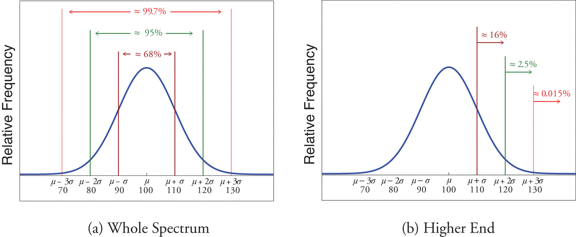
- Since \(68\%\) of the IQ scores lie within the interval from \(90\) to \(110\), it must be the case that \(32\%\) lie outside that interval. By symmetry approximately half of that \(32\%\), or \(16\%\) of all IQ scores, will lie above \(110\). If \(16\%\) lie above \(110\), then \(84\%\) lie below. We conclude that the IQ score \(110\) is the \(84^{th}\) percentile.
- The same analysis applies to the score \(120\). Since approximately \(95\%\) of all IQ scores lie within the interval form \(80\) to \(120\), only \(5\%\) lie outside it, and half of them, or \(2.5\%\) of all scores, are above \(120\). The IQ score \(120\) is thus higher than \(97.5\%\) of all IQ scores, and is quite a high score.
- By a similar argument, only \(15/100\) of \(1\%\) of all adults, or about one or two in every thousand, would have an IQ score above \(130\). This fact makes the score \(130\) extremely high.
Chebyshev’s Theorem
The Empirical Rule does not apply to all data sets, only to those that are bell-shaped, and even then is stated in terms of approximations. A result that applies to every data set is known as Chebyshev’s Theorem.
For any numerical data set,
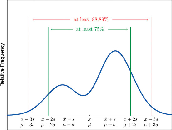
- at least \(3/4\) of the data lie within two standard deviations of the mean, that is, in the interval with endpoints \(\bar{x}\pm 2s\) for samples and with endpoints \(\mu \pm 2\sigma\) for populations;
- at least \(8/9\) of the data lie within three standard deviations of the mean, that is, in the interval with endpoints \(\bar{x}\pm 3s\) for samples and with endpoints \(\mu \pm 3\sigma\) for populations;
- at least \(1-1/k^2\) of the data lie within \(k\) standard deviations of the mean, that is, in the interval with endpoints \(\bar{x}\pm ks\) for samples and with endpoints \(\mu \pm k\sigma\) for populations, where \(k\) is any positive whole number that is greater than \(1\).
Figure \(\PageIndex{4}\) gives a visual illustration of Chebyshev’s Theorem.
It is important to pay careful attention to the words “at least” at the beginning of each of the three parts of Chebyshev’s Theorem. The theorem gives the minimum proportion of the data which must lie within a given number of standard deviations of the mean; the true proportions found within the indicated regions could be greater than what the theorem guarantees.
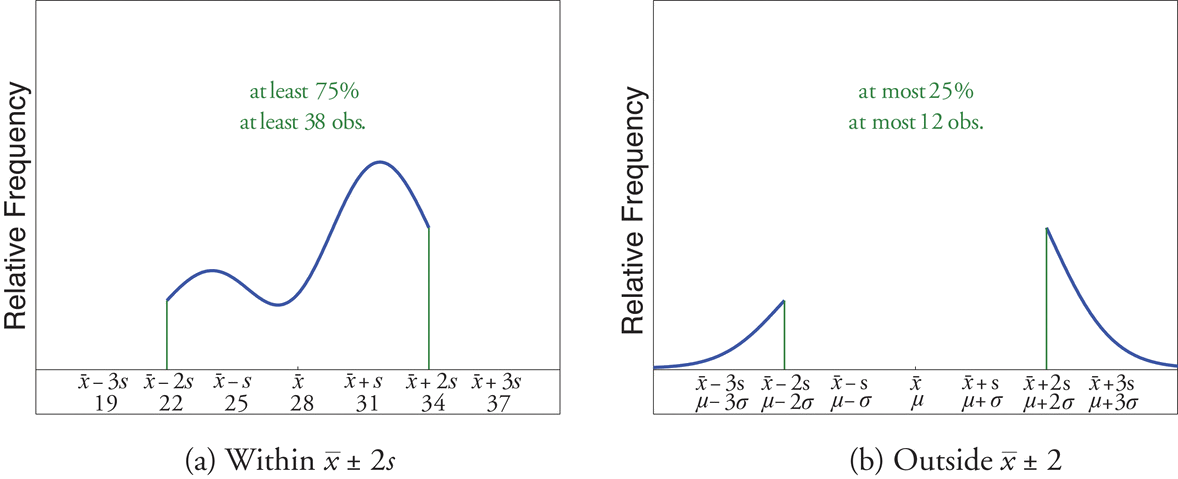
A sample of size \(n=50\) has mean \(\bar{x}=28\) and standard deviation \(s=3\). Without knowing anything else about the sample, what can be said about the number of observations that lie in the interval \((22,34)\)? What can be said about the number of observations that lie outside that interval?
Solution
The interval \((22,34)\) is the one that is formed by adding and subtracting two standard deviations from the mean. By Chebyshev’s Theorem, at least \(3/4\) of the data are within this interval. Since \(3/4\) of \(50\) is \(37.5\), this means that at least \(37.5\) observations are in the interval. But one cannot take a fractional observation, so we conclude that at least \(38\) observations must lie inside the interval \((22,34)\).
If at least \(3/4\) of the observations are in the interval, then at most \(1/4\) of them are outside it. Since \(1/4\) of \(50\) is \(12.5\), at most \(12.5\) observations are outside the interval. Since again a fraction of an observation is impossible, \(x\; (22,34)\).
The number of vehicles passing through a busy intersection between \(8:00\; a.m.\) and \(10:00\; a.m.\) was observed and recorded on every weekday morning of the last year. The data set contains \(n=251\) numbers. The sample mean is \(\bar{x}=725\) and the sample standard deviation is \(s=25\). Identify which of the following statements must be true.
- On approximately \(95\%\) of the weekday mornings last year the number of vehicles passing through the intersection from \(8:00\; a.m.\) to \(10:00\; a.m.\) was between \(675\) and \(775\).
- On at least \(75\%\) of the weekday mornings last year the number of vehicles passing through the intersection from \(8:00\; a.m.\) to \(10:00\; a.m.\) was between \(675\) and \(775\).
- On at least \(189\) weekday mornings last year the number of vehicles passing through the intersection from \(8:00\; a.m.\) to \(10:00\; a.m.\) was between \(675\) and \(775\).
- On at most \(25\%\) of the weekday mornings last year the number of vehicles passing through the intersection from \(8:00\; a.m.\) to \(10:00\; a.m.\) was either less than \(675\) or greater than \(775\).
- On at most \(12.5\%\) of the weekday mornings last year the number of vehicles passing through the intersection from \(8:00\; a.m.\) to \(10:00\; a.m.\) was less than \(675\).
- On at most \(25\%\) of the weekday mornings last year the number of vehicles passing through the intersection from \(8:00\; a.m.\) to \(10:00\; a.m.\) was less than \(675\).
Solution
- Since it is not stated that the relative frequency histogram of the data is bell-shaped, the Empirical Rule does not apply. Statement (1) is based on the Empirical Rule and therefore it might not be correct.
- Statement (2) is a direct application of part (1) of Chebyshev’s Theorem because \(\bar{x}-2s\), \(\bar{x}+2s = (675,775)\). It must be correct.
- Statement (3) says the same thing as statement (2) because \(75\%\) of \(251\) is \(188.25\), so the minimum whole number of observations in this interval is \(189\). Thus statement (3) is definitely correct.
- Statement (4) says the same thing as statement (2) but in different words, and therefore is definitely correct.
- Statement (4), which is definitely correct, states that at most \(25\%\) of the time either fewer than \(675\) or more than \(775\) vehicles passed through the intersection. Statement (5) says that half of that \(25\%\) corresponds to days of light traffic. This would be correct if the relative frequency histogram of the data were known to be symmetric. But this is not stated; perhaps all of the observations outside the interval (\(675,775\)) are less than \(75\). Thus statement (5) might not be correct.
- Statement (4) is definitely correct and statement (4) implies statement (6): even if every measurement that is outside the interval (\(675,775\)) is less than \(675\) (which is conceivable, since symmetry is not known to hold), even so at most \(25\%\) of all observations are less than \(675\). Thus statement (6) must definitely be correct.
Key Takeaway
- The Empirical Rule is an approximation that applies only to data sets with a bell-shaped relative frequency histogram. It estimates the proportion of the measurements that lie within one, two, and three standard deviations of the mean.
- Chebyshev’s Theorem is a fact that applies to all possible data sets. It describes the minimum proportion of the measurements that lie must within one, two, or more standard deviations of the mean.