10.6: Test of Mean vs. Hypothesized Value – A Complete Example

Last updated
Save as PDF

Page ID: 20909

\( \newcommand{\vecs}[1]{\overset { \scriptstyle \rightharpoonup} {\mathbf{#1}} } \) \( \newcommand{\vecd}[1]{\overset{-\!-\!\rightharpoonup}{\vphantom{a}\smash {#1}}} \)\(\newcommand{\id}{\mathrm{id}}\) \( \newcommand{\Span}{\mathrm{span}}\) \( \newcommand{\kernel}{\mathrm{null}\,}\) \( \newcommand{\range}{\mathrm{range}\,}\) \( \newcommand{\RealPart}{\mathrm{Re}}\) \( \newcommand{\ImaginaryPart}{\mathrm{Im}}\) \( \newcommand{\Argument}{\mathrm{Arg}}\) \( \newcommand{\norm}[1]{\| #1 \|}\) \( \newcommand{\inner}[2]{\langle #1, #2 \rangle}\) \( \newcommand{\Span}{\mathrm{span}}\) \(\newcommand{\id}{\mathrm{id}}\) \( \newcommand{\Span}{\mathrm{span}}\) \( \newcommand{\kernel}{\mathrm{null}\,}\) \( \newcommand{\range}{\mathrm{range}\,}\) \( \newcommand{\RealPart}{\mathrm{Re}}\) \( \newcommand{\ImaginaryPart}{\mathrm{Im}}\) \( \newcommand{\Argument}{\mathrm{Arg}}\) \( \newcommand{\norm}[1]{\| #1 \|}\) \( \newcommand{\inner}[2]{\langle #1, #2 \rangle}\) \( \newcommand{\Span}{\mathrm{span}}\)\(\newcommand{\AA}{\unicode[.8,0]{x212B}}\)

Example – Soy sauce production

A food company has a policy that the stated contents of a product match the actual results. A General Question might be “Does the stated net weight of a food product match the actual weight?” The quality control statistician decides to test the 16 ounce bottle of Soy Sauce and must now design the experiment.

The quality‐control statistician has been given the authority to sample 36 bottles of soy sauce and knows from past testing that the population standard deviation is 0.5 ounces. The model will be a test of population mean vs. hypothesized value of 16 oz. A two‐tailed test is selected since the company is concerned about both overfilling and underfilling the bottles as the stated policy is that the stated weight should match the actual weight of the product.

Research Hypotheses:

\(H_o: \mu =16\) (The filling machine is operating properly)

\(H_a: \mu \neq 16\) (The filling machine is not operating properly)

Since the population standard deviation is known the test statistic will be \(Z=\dfrac{\overline{X}-\mu}{\sigma / \sqrt{n}}\). This model is appropriate since the sample size assures that the distribution of the sample mean is approximately Normal due to the Central Limit Theorem.

Type I error would be to reject the Null Hypothesis and say that the machine is not running properly when in fact it was operating properly. Since the company does not want to needlessly stop production and recalibrate the machine, the statistician chooses to limit the probability of Type I error by setting the level of significance (\(\alpha\)) to 5%.

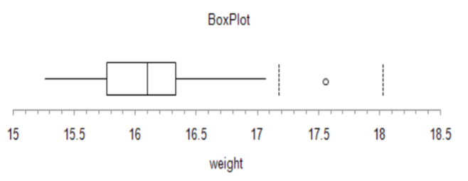
The statistician now conducts the experiment and samples 36 bottles over one hour and determines from a box plot of the data that there is one unusual observation of 17.56 ounces. The value is rechecked and kept in the data set.

Next, the sample mean and the test statistic are calculated.

\[\overline{X}=16.12 \text { ounces } \qquad \qquad Z=\dfrac{16.12-16}{0.5 / \sqrt{36}}=1.44 \nonumber \]

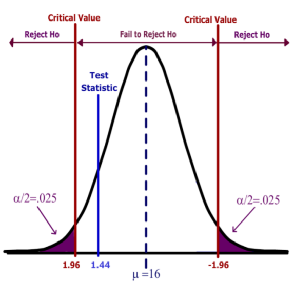
The decision rule under the critical value method would be to reject the Null Hypothesis when the value of the test statistic is in the rejection region. In other words, reject \(H_o\) when \(Z >1.96\) or \(Z<‐1.96\).

Based on this result, the decision is fail to reject \(H_o\), since the test statistic does not fall in the rejection region.

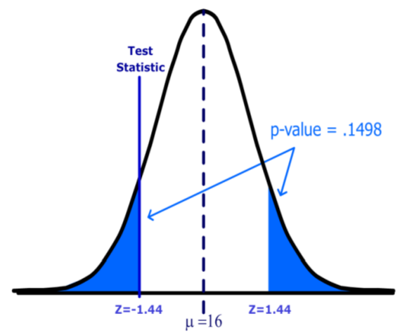
Alternatively (and preferably) the statistician could use the p‐value method of decision rule. The \(p\)‐value for a two‐tailed test must include all values (positive and negative) more extreme than the Test Statistic, so in this example we find the probability that \(Z < ‐1.44\) or \(Z > 1.44\) (the area shaded blue).

Using a calculator, computer software or a Standard Normal table, the \(p\)‐value=0.1498. Since the \(p\)‐value is greater than \(\alpha\) the decision again is fail to reject \(H_o\).

Finally the statistician must report the conclusions and make a recommendation to the company’s management:

“There is insufficient evidence to conclude that the machine that fills 16 ounce soy sauce bottles is operating improperly. This conclusion is based on 36 measurements taken during a single hour’s production run. I recommend continued monitoring of the machine during different employee shifts to account for the possibility of potential human error”.

The statistician makes the weak statement and is not stating that the machine is running properly, only that there is not enough evidence to state that the machine is running improperly. The statistician also reports concerns about the sampling of only one shift of employees (restricting the inference to the sampled population) and recommends repeating the experiment over several shifts.