2: Kernel Density Estimation (KDE)

2.1: Concept of Naive Bayes Classifier

Given an vector \(\textbf{x}\) = \((x_{1},...,x_{m})^T\), We assign the probability \[\begin{aligned} & P(C_k|x_{1},...x_{m}) \end{aligned}\] to the event that the observation \(x_i\) belongs to the class \(C_k\).

Here we assume each feature is conditionally independent of every other feature given the class variable. Then, we use the Bayes’ theorem to calculate the probability as follows:

\[\begin{aligned} P(C_k|x_{1},...x_{m}) & =\frac{P(C_k)P(\textbf{x}|C_k)}{P(\textbf{x})}\\ & = \frac{P(C_k)\prod_{i = 1}^{m}P(x_{i}|C_k)}{P(\textbf{x})}, \end{aligned}\]

Due to the independent assumption, we can write the likelihood function as

\[P(\textbf{x}|C_k) = \prod_{i=1}^{m} P(x_i|C_k)\]

Since the denominator \(P(\textbf{x})\), which is in the Bayes Theorem doesn’t depend on \(C_k\), so, we can treat the denominator as a constant. So, we rewrite the Bayes Theorem as

\[P(C_k|\textbf{x}) \propto P(C_k)\prod_{i=1}^{m} P(x_i|C_k)\]

Hence the Naive Bayes classfier is the following function to assgin the label to the observation:

\[\begin{aligned} \hat{y} = \underset{k \in \{1,...,K\}}{argmax}P(C_k)\prod_{i = 1}^{m}P(x_{i}|C_k) \end{aligned}\]

Next, we want to know how to calculate the conditional probability \(p(x_i|C_k)\). Here are two common ways.

2.2: Density Estimation

2.2.1: Parametric Method

A common assumption is that, within each class, the values of numeric features are normally distributed. So, we can write \(p(x_i|C_k) = g(x_i;\mu_{C_k},\sigma_{C_k})\), where \(g(x;\mu,\sigma) = \frac{1}{(2\pi\sigma^{2})^{\frac{1}{2}}}e^{\frac{-(x-\mu)^2}{2\sigma^{2}}}\), is the p.d.f for the normal distribution. Here, the \(\mu_{C_k}\) and \(\sigma_{C_k}\) could be get through maximum likelihood estimation.

2.2.2: Non-parametric Method

Firstly, we can use histogram. The idea of this method is straight forward. We consider there is a \(h > 0\) as a bandwidth near \(x_0\). And we denote \(\hat{f}(x)\) as the probability density function of our observations and \(F(x)\) as the cumulative density function. Thus, by the definition of derivative, at the point \(x_0\),

\[\hat{f}(x_0) = \frac{F(x_0 + \frac{h}{2}) - F(x_0 - \frac{h}{2})}{h}\]

Since our numerator

\[F(x_0 + \frac{h}{2}) - F(x_0 - \frac{h}{2}) = P(x_0-\frac{h}{2} \leq x \leq x_0 + \frac{h}{2}) \]

we can write our numerator as \(\frac{\# x_i \in N(x_0)}{n}\). So, we can estimate the probability at \(x_0\) as \[\hat{f}(x_0) = \frac{\# x_i \in N(x_0)}{nh}\] But as the following plot shows, this kind of method

Next, we use the kernel density estimation to make the plot smooth. Suppose in the class \(C_k\), we have p features, and in each feature, \((x_1,x_2,...,x_n)\) be an independent and identically distributed sample drawn from some distribution with an unknown density f. Then, its kernel density estimator can be drawn as follows,

\[\hat{f_h}(x) = \frac{1}{nh}\sum_{i=1}^{n}K(\frac{x-x_i}{h})\]

where and \(h > 0\) is a smoothing parameter called the bandwidth, and \(K(u))\) is the kernel function with the properties that

\[\int_{-\infty}^{\infty}K(u)du = 1 \quad \textrm{and} \quad E(u)=0\]

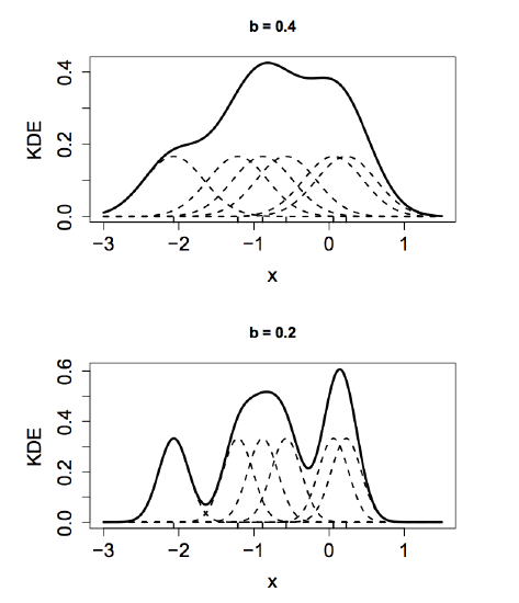
y using kernel density estimation, we can also get the p.d.f of every feature in each class. Here, the choice of \(K\) is not crucial, but the choice of bandwidth \(h\) is important. There is a bias-variance tradeoff in the selection of \(h\) as shown in the following graph.

Write \(K_h(x, X) = h^{-1} K ((x-X)/h)\) and \(\hat{f}(x)=n^{-1} \sum_i K_h (x, X_i)\). Thus, \(E(\hat{f_n}(x)) = E(K_h (x,X))\) and \(V(\hat{f_n}(x)) = n^{-1} V(K_h(x,X)) \). Now, \[E[K_h(x,X)] = \int \frac{1}{h} K(\frac{x-t}{h}) f(t)dt\] \[= \int K(u)f(x-hu)du\] \[= \int K(u) [f(x) -huf'(x) + \frac{h^2 u^2}{2} f''(x) + ... ]du\] \[= f(x) + \frac{1}{2} h^2 f''(x) \int u^2 K(u)du ...\] since \(\int K(x)dx=1\) and \(\int x K(x)dx=0\). The bias is \[E[K_h (x,X)]-f(x)=\frac{1}{2}\sigma^2_k h^2 f''(x) + O(h^4)\] By a similar calculation, \[V[\hat{f_n}(x)] = \frac{f(x) \int K^2(x)dx}{nh} + O(\frac{1}{n})\] If the \(h\) is small, bias is small and variance is large. However, if the \(h\) is wide, variance is small due to the effects of averaging, but bias is large, since we use more observations further from the target \(x\).