1: Support Vector Machine (SVM)

1.1 Basic Background of SVM

The idea for Support Vector Machine is straight forward: Given observations $x_i \in {\rm I\!R}^p$, $i \in 1,...,n$, and each observation $x_i$ has a class $y_i$, where $y_i \in \{-1,1\}$, we want to find a hyperplane such that it can separate the observations based on their classes and also maximize the the minimum distance of the observation to the hyperplane.

First, we denote the best hyperplane as $w^Tx+b = 0$. From the linear algebra, we know the distance from a point $x_0$ to the plane $w^Tx+b = 0$ is calculated by: $$\begin{aligned} \text{Distance} = \dfrac{|w^Tx_0 + b|}{||w||} \end{aligned}$$ Then we want such hyperplane can correctly separate two classes, which is equivalent to satisfy following restrictions:

$$\begin{aligned} &(w^Tx_i+b) > 0, & & \text{if $y_i$ = 1} \\ &(w^Tx_i+b) < 0, & & \text{if $y_i$ = -1}, \end{aligned}$$

which is equivalent to $$\begin{aligned} &y_i(w^Tx_i+b) > 0, & &i = 1, \ldots, n. \end{aligned}$$

Our goal is to maximize the minimum distance for all observations to that hyperplane,so we have our first optimization problem: $$\begin{aligned} &\underset{w,b}{\text{maximize}} & & \text{min} \{\frac{|w^Tx_i+b|}{||w||}\}\\ & \text{s.t.} & & y_i(w^Tx_i+b) > 0,i = 1, \ldots, n. \end{aligned}$$

Then we define margin $M = \text{min}\{\frac{|w^Tx_i+b|}{||w||}\}$, and for the mathematics convenience, we scale $w$ such that satisfy $||w|| = 1$

$$\begin{aligned} &\underset{w,||w|| = 1,b}{\text{maximize}} & & M\\ & \text{ s.t.} & & y_i(w^Tx_i+b) \geq M, i = 1, \ldots, n. \end{aligned}$$

Then we define $v = \frac{w}{M}$ and the norm of the $||v||$ is therefore $\frac{1}{M}$. We substitute $v$ back to our optimization:

$$\begin{aligned} &\underset{v,b}{\text{maximize}} & & \frac{1}{||v||}\\ & \text{s.t.} & & y_i(\frac{w^T}{M}x_i+\frac{b}{M}) \geq \frac{M}{M} = 1, i = 1, \ldots, n. \end{aligned}$$

Then we change the variable name v to w, and to maximize $\frac{1}{||v||}$ is equivalent to minimize $\frac{1}{2}w^Tw$. So we get our final optimization problem as:

$$\begin{aligned} &\underset{w,b}{\text{minimize}} & & \frac{1}{2}w^Tw\\ & \text{s.t.} & & y_i(w^Tx_i+b) \geq 1, i = 1, \ldots, n. \end{aligned}$$

We want to use the Method of Lagrange Multipliers to solve the optimization problem. We can write our constrained as $g_i(w) = y_i(w^T x_i+b) - 1 \geq 0$. Lets define $L(w,b,\alpha \geq 0) = \frac{1}{2}w^Tw - \sum_{i=1}^{n}\alpha_i[y_i(w^Twx_i+b) -1]$. We observe that the maximum of the function $L$ with respect to $\alpha$ equals $\frac{1}{2}w^Tw$. So we change our original optimization problem to the new one : $$\begin{aligned} &\underset{w,b}{\text{min }} \underset{\alpha \geq 0}{\text{max }}L(w,b,\alpha) = \frac{1}{2}w^Tw - \sum_{i=1}^{n}\alpha_i[y_i(w^Twx_i+b) -1] \end{aligned}$$ where $\alpha$ is the Lagrange Multiplier.

We can verify that $w,b,\alpha$ satisfy Karush-Kuhn-Tucker (KKT condition). Therefore, we can solve the primal problem by solving its dual problem: $$\begin{aligned} &\underset{\alpha \geq 0}{\text{max }}\underset{w,b}{\text{min }} L(w,b,\alpha) = \frac{1}{2}w^Tw - \sum_{i=1}^{n}\alpha_i[y_i(w^Twx_i+b) -1] \end{aligned}$$

To solve the dual problem, we first need to set the partial derivative of L(w,b,$\alpha$) with respect of w and b to 0: $$\begin{aligned} & \nabla_w L(w,b,\alpha)= w - \sum_{i = 1}^{n}\alpha_iy_ix_i = 0\\ & \frac{\partial}{\partial b}L(w,b,\alpha)= \sum_{i=1}^{n}\alpha_iy_i= 0 \end{aligned}$$

Then we substitute them back to the function L(w,b,$\alpha$) $$\begin{aligned} L(w,b,\alpha) & =\frac{1}{2}w^Tw-\sum_{i = 1}^{n}\alpha_i(y_i(w^Tx_i+b)-1)\\ & = \frac{1}{2}w^Tw - \sum_{i = 1}^{n}\alpha_iy_iw^Tx_i - \sum_{i = 1}^{n}\alpha_iy_ib + \sum_{i = 1}^{n}\alpha_i\\ & = \frac{1}{2}w^T\sum_{i = 1}^{n}\alpha_iy_ix_i - w^T\sum_{i = 1}^{n}\alpha_iy_ix_i - b\sum_{i = 1}^{n}\alpha_iy_i + \sum_{i = 1}^{n}\alpha_i\\ & = -\frac{1}{2}w^T\sum_{i = 1}^{n}\alpha_iy_ix_i - b\sum_{i = 1}^{n}\alpha_iy_i + \sum_{i = 1}^{n}\alpha_i \\ & = -\frac{1}{2}(\sum_{i = 1}^{n}\alpha_iy_ix_i)^T\sum_{i = 1}^{n}\alpha_iy_ix_i - b\sum_{i = 1}^{n}\alpha_iy_i + \sum_{i = 1}^{n}\alpha_i \\ & = -\frac{1}{2}\sum_{i = 1}^{n}\alpha_iy_i(x_i)^T\sum_{i = 1}^{n}\alpha_iy_ix_i - b\sum_{i = 1}^{n}\alpha_iy_i + \sum_{i = 1}^{n}\alpha_i \\ & = -\frac{1}{2}\sum_{i,j = 1}^{n}\alpha_i\alpha_jy_iy_jx_i^Tx_j - b\sum_{i = 1}^{n}\alpha_iy_i + \sum_{i = 1}^{n}\alpha_i \\ & = -\frac{1}{2}\sum_{i,j = 1}^{n}\alpha_i\alpha_jy_iy_jx_i^Tx_j + \sum_{i = 1}^{n}\alpha_i \\ \end{aligned}$$

and simplify the dual problem as: $$\begin{aligned} \underset{\alpha \geq 0}{\text{maximize }} & W(\alpha) = \sum_{i = 1}^{n}\alpha_i - \frac{1}{2}\sum_{i,j=1}^{n}y_iy_j\alpha_i\alpha_j<x_i,x_j> \\ \text{s.t.} & \sum_{i = 1}^{n}\alpha_iy_i = 0 \end{aligned}$$

Then we notice that it is a convex optimization problem so that we can use SMO algorithm to solve the value of Lagrange multiplier $\alpha$. And using formula (5), we can compute the parameter $w$. Also,b is calculated as $$\begin{aligned} b = \frac{min_{i:y_i = 1}{w^Tx_i} - max_{i:y_i = -1}{w^Tx_i}}{2} \end{aligned}$$

Therefore, after figuring out the parameter $w$ and $b$ for the best hyperplane, for the new observation $x_i$, the decision rule is that $$\begin{aligned} & y_i = {\begin{cases} 1, & \text{for } w^Tx_i+b \geq 1\\ -1, & \text{for } w^Tx_i+b \leq 1\\ \end{cases}} \end{aligned}$$

1.2 Soft Margin

In most real-world data, hyperplane cannot totally separate binary classes data, so we are tolerant to some observations in train data at wrong side of margin or hyperplane. We called the margin in above situation as Soft Margin or Support Vector Classifier.Here is primal optimization problem of Soft Margin:
$$\begin{aligned} & \underset{w,b,\varepsilon_i}{\text{minimize}} & & \frac{1}{2}w^Tw + C\sum_{i = 1}^{n}\varepsilon_i\\ & \text{s.t.} & & y_i(w^Tx_i+b) \geq 1 - \varepsilon_i,\; \text{and } \varepsilon_i \geq 0, i = 1, \ldots, n, \end{aligned}$$

where $\xi_i$ is the slack variables that allow misclassification; the penalty term $\sum_{i=1}^{l}\xi_i$ is a measure of the total number of misclassification in the model constructed by training dataset; C,a tuning parameter, is the misclassification cost that controls the trade-off of maximizing the margin and minimizing the penalty term.
Following the same process we have done in deriving the hard margin,We can solve the primal problem by proceed it in its dual space. Here is the Lagrangian of (9) and the $\alpha_i$ and $\beta_i$ showing below are the Lagrange Multiplier:
$$\begin{aligned} \underset{w,b,\varepsilon_i}{\text{min }}\underset{\alpha \geq 0, \beta \geq 0}{\text{max }}L(w,b,\alpha, \beta,\varepsilon) &= \frac{1}{2}||w||^2 +C\sum\limits_{i=1}^{n}\varepsilon_{i}-\sum\limits_{i=1}^{n} \alpha_{i} [y_{i}({w}^T \cdot {x}_{i} + b)- 1+\varepsilon_{i}] -\sum\limits_{i=1}^{n}\beta_{i}\varepsilon_{i} , \\ \end{aligned}$$

Due to the nonnegative property of the primal constraints and Lagrange Multiplier, the part $-\sum\limits_{i=1}^{n} \alpha_{i} [y_{i}({w}^T \cdot \vec{x}_{i} + b) - 1+\varepsilon_{i}] -\sum\limits_{i=1}^{n}\beta_{i}\varepsilon_{i}$ should be negative. thus we can minimize that part to zero in order to get $\underset{\alpha \geq 0, \beta \geq 0}{\text{max }}L(w,b,\alpha, \beta,\varepsilon) = \frac{1}{2}||w||^2 +C\sum\limits_{i=1}^{n}\varepsilon_{i}-\sum\limits_{i=1}^{n} \alpha_{i} [y_{i}({w}^T \cdot {x}_{i} + b) - 1+\varepsilon_{i}] -\sum\limits_{i=1}^{n}\beta_{i}\varepsilon_{i}$ with respect to w, b and $\varepsilon$. However, the constraints $\alpha \geq 0$ and $\beta \geq 0$ make it difficult to find the maximization. Therefore, we transform the primal problem to the following dual problem through the KKT condition:

$$\begin{aligned} \underset{\alpha \geq 0, \beta \geq 0} {\text{max}}\underset{w,b,\varepsilon_i}{\text{min }}L(w,b,\alpha, \beta,\varepsilon) &= \frac{1}{2}||w||^2 +C\sum\limits_{i=1}^{n}\varepsilon_{i}-\sum\limits_{i=1}^{n} \alpha_{i} [y_{i}({w}^T \cdot {x}_{i} + b)- 1+\varepsilon_{i}] -\sum\limits_{i=1}^{n}\beta_{i}\varepsilon_{i} , \\ \end{aligned}$$

Because the subproblem for minimizing the equation with respect to w, b and $\varepsilon$, we have no constraints on them, thus we could set the gradient to 0 as follows to find $\underset{w,b,\varepsilon_i}{\text{min }}L(w,b,\alpha, \beta,\varepsilon)$:
$$\begin{aligned} \nabla_w L &= \vec{w} - \sum\limits_{i=1}^{n} \alpha_{i} y_{i} x_{i}=0 \Rightarrow \vec{w} = \sum\limits_{i=1}^{n} \alpha_{i} y_{i} x_{i}\\ \frac{\partial L}{\partial b} &= - \sum\limits_{i=1}^{n} y_{i} x_{i}= 0 \Rightarrow \sum\limits_{i=1}^{n} y_{i} x_{i}=0\\ \frac{\partial L}{\partial \varepsilon_{i}} &= C- \alpha_{i} - \beta_{i}=0, \Rightarrow C = \alpha_{i}+\beta_{i}\\ \end{aligned}$$

When we plug Equation set $(12)$ to Equation $(11)$, we get the dual Lagrangian form of this optimization problem as follows:
$$\begin{aligned} &\mathop{max}_{\alpha_i \geq 0} && \sum\limits_{i=1}^{n} \alpha_{i} - \frac{1}{2}\sum\limits_{i=1}^{n}\sum\limits_{j=1}^{n} \alpha_{i}\alpha_{j}y_{i}y_{j}{x}_{i}^T{x}_{j} \\ &s.t. && \sum_{i=1}^{n} y_i \alpha_i = 0 \text{ and } 0 \leq \alpha_i \leq C, \text{for } i = 1,...,n \end{aligned}$$
Finally, the decision rule will show as follows:
$(1)$ If $\alpha_{i} = 0$ and $\varepsilon_{i} = 0$, the testing observation $x_{i}$ has been classified on the right side.
$(2)$ If $0 < \alpha_{i} < C$, we can conclude that $\varepsilon_{i} = 0$ and $y_{i}={w}^T\cdot\vec{x}_{i} + b$, which means the testing observation $x_{i}$ is a support vector.
$(3)$ If $\alpha_{i} = 0$, $\varepsilon_{i} >0$ and $x_{i}$ is a support vector, we can conclude that $x_{i}$ is correctly classified when $0 \leq \varepsilon_{i} < 1$, and $x_{i}$ is misclassified when $\varepsilon_{i} > 1$.

1.3: Kernel Method

Since we calculate $w=\sum_{i=1}^{n}\alpha_iy_ix_i$, so our hyperplane can be rewrite as $$g(x) = (\sum_{i=1}^{n}\alpha_iy_ix_i)^{T}x + b = \sum_{i=1}^{n}\alpha_iy_i<x_i,x> + b$$ where $<x_i,x>$ represents the inner product of $x_i$ and $x$. What we discussed above is about linear separable. What if our data set is not linear separable? One common way here is define a map as: $$\phi:\mathbb{R}^p\to\mathbb{R}^m$$ A feature mapping $\phi$, for instance, could be $$\begin{aligned} & \phi(x) = \begin{bmatrix}x \\x^2 \\ x^3 \end{bmatrix}. \end{aligned}$$

The idea is that if the observations are inseparable in current feature space, we can use a feature mapping function $\phi$ and try to separate the observations after being mapped.

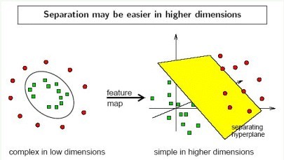
Here is a plot shows how the mapping function $\phi$ works.

Hence, in order to solve the hyperplane to separate the observations after being mapped, we simply replace x with $\phi(x)$ everywhere in the previous optimization problem and get:

$$\begin{aligned} &\underset{w,b}{\text{maximize}} & & \frac{1}{2}w^Tw\\ & \text{s.t.} & & y_i(w^T\phi(x_i)+b) \geq 1, i = 1, \ldots, n. \end{aligned}$$

From the previous part, we know that for each observations, we only need their pairwise inner products to solve the problem. But since computing the inner product in high dimensional space is expensive or even impossible, we need another way to computing the inner product.So here, given a feature mapping $\phi(x)$ we define the corresponding Kernel function K as:

$$\begin{aligned} K(x_i,x_j) = \phi(x_i)^T\phi(x_j) = <\phi(x_i),\phi(x_j)> \end{aligned}$$

So now, instead of actually computing the inner product of pairwise observations, we use the kernel function to help us in computation. And using the same methods as before, we can get our hyperplane as:

$$\begin{aligned} w = \sum_{i=1}^{n}\alpha_iy_i\phi(x_i), \end{aligned}$$

and $$\begin{aligned} b = \frac{min_{i:y_i = 1}\sum_{j=1}^{n}\alpha_iy_iK(x_i,x_j) - max_{i:y_i = -1}\sum_{j=1}^{n}\alpha_iy_iK(x_i,x_j)}{2} \end{aligned}$$

So after using kernel, our decision rule becomes: $$\begin{aligned} & y_i = {\begin{cases} 1, & \text{for } \sum_{i=1}^{n}\alpha_iy_i<\phi(x_i),\phi(x)> + b \geq 1\\ -1, & \text{for } \sum_{i=1}^{n}\alpha_iy_i<\phi(x_i),\phi(x)> + b \leq 1\\ \end{cases}} \end{aligned}$$

There are some commonly used kernel: Polynomial Kernel and Gaussian Kernel. Polynomial kernel with degree n is defined as $K(x_i,x_j) = (x_i^Tx_j)^d$ and Gaussian kernel with $\sigma$ as $K(x_i,x_j) = \text{exp}{-\frac{||x_i-x_j||^2}{2\sigma^2}}$.