The Monte Carlo Simulation Method

Last updated
Save as PDF

Page ID: 977

\( \newcommand{\vecs}[1]{\overset { \scriptstyle \rightharpoonup} {\mathbf{#1}} } \) \( \newcommand{\vecd}[1]{\overset{-\!-\!\rightharpoonup}{\vphantom{a}\smash {#1}}} \)\(\newcommand{\id}{\mathrm{id}}\) \( \newcommand{\Span}{\mathrm{span}}\) \( \newcommand{\kernel}{\mathrm{null}\,}\) \( \newcommand{\range}{\mathrm{range}\,}\) \( \newcommand{\RealPart}{\mathrm{Re}}\) \( \newcommand{\ImaginaryPart}{\mathrm{Im}}\) \( \newcommand{\Argument}{\mathrm{Arg}}\) \( \newcommand{\norm}[1]{\| #1 \|}\) \( \newcommand{\inner}[2]{\langle #1, #2 \rangle}\) \( \newcommand{\Span}{\mathrm{span}}\) \(\newcommand{\id}{\mathrm{id}}\) \( \newcommand{\Span}{\mathrm{span}}\) \( \newcommand{\kernel}{\mathrm{null}\,}\) \( \newcommand{\range}{\mathrm{range}\,}\) \( \newcommand{\RealPart}{\mathrm{Re}}\) \( \newcommand{\ImaginaryPart}{\mathrm{Im}}\) \( \newcommand{\Argument}{\mathrm{Arg}}\) \( \newcommand{\norm}[1]{\| #1 \|}\) \( \newcommand{\inner}[2]{\langle #1, #2 \rangle}\) \( \newcommand{\Span}{\mathrm{span}}\)\(\newcommand{\AA}{\unicode[.8,0]{x212B}}\)

What is Monte Carlo?

In this section, we will discuss some aspects of the Monte Carlo method our team used to simulate high dimensional data. The Monte Carlo methods are basically a class of computational algorithms that rely on repeated random sampling to obtain certain numerical results, and can be used to solve problems that have a probabilistic interpretation. This method of simulation is useful for our project because it enables us to sample high-dimensional vectors from a known distribution--the standard normal distribution--so that we can compare our simulated results with our theory. Although using real high-dimensional data is also an option, we more often than not do not know the true distribution of these data points, so what we observe from real data might not always align nicely with theory. However, with simulated data, we can always test to see if what we're expecting is correct if we fix a sample size, dimension, and distribution beforehand.

How does it work?

Monte Carlo simulation works by selecting a random value for each task, and then building models based on those values. This process is then repeated many times, with different values so in the end, the output is a distribution of outcomes.

Below we have two common examples, CLT and LLN, that utilizes this Monte Carlo simulation method.

CLT

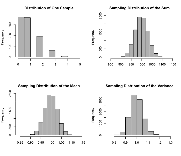
The Central Limit Theorem (CLT) is a way to approximate the probability of the sample average is close to the mean. When a random sample of size n is taken from any distribution with mean u and variance \( \sigma^2 \), the sample mean will have a distribution approximately Normal with mean u and variance \( \sigma^2/n \). It doesn't matter what the shape of the underlying distribution is, all that is necessary is finite variance and many, many repeated samples of size n from a population. Then, the average or sum will be approximately Normal distributed. Alternatively, the sum will be approximately Normal with mean \(\mu\) and variance \( n\sigma^2 \).

The CLT can be demonstrated through simulation. Below demonstrates the CLT theorem using Poisson distribution with sample size 1000.

Another example below is Exponential distribution with sample size 10,000.

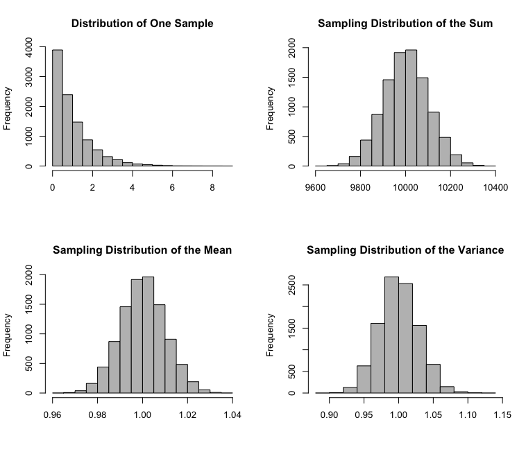
As from these example plots with varying sample sizes and distributions, the data's sample mean still has approximately a Normal distribution.

The R code is below, and one can adjust the parameters to test the theorem.

# Central Limit Theorem Simulation
# n: sample size of each sample
# dist: underlying distribution where the sample is drawn

simulation <- function(n, dist=NULL, param1=NULL, param2=NULL) {
r <- 10000 # Number of replications/samples - (DO NOT ADJUST)
# This produces a matrix of observations with
# n columns and r rows. Each row is one sample:
my.samples <- switch(dist,
"E" = matrix(rexp(n*r,param1),r),
"N" = matrix(rnorm(n*r,param1,param2),r),
"U" = matrix(runif(n*r,param1,param2),r),
"P" = matrix(rpois(n*r,param1),r),
"C" = matrix(rcauchy(n*r,param1,param2),r),
"B" = matrix(rbinom(n*r,param1,param2),r),
"G" = matrix(rgamma(n*r,param1,param2),r),
"X" = matrix(rchisq(n*r,param1),r),
"T" = matrix(rt(n*r,param1),r))
all.sample.sums <- apply(my.samples,1,sum)
all.sample.means <- apply(my.samples,1,mean)
all.sample.vars <- apply(my.samples,1,var)
par(mfrow=c(2,2))
hist(my.samples[1,], col="gray", main="Distribution of One Sample", xlab="")
hist(all.sample.sums, col="gray", main="Sampling Distribution of the Sum", xlab="")
hist(all.sample.means,col="gray", main="Sampling Distribution of the Mean", xlab="")
hist(all.sample.vars,col="gray", main="Sampling Distribution of the Variance", xlab="")
}

simulation(n=1000, dist="P", param1=1)

simulation(n=10000, dist="E", param1=1)

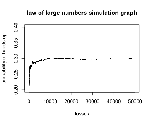
LLN

The Law of Large Numbers (LLN) is a way to explain how the average of a large sample of independently and identically distributed (iid) random variables will be close to their mean.

An example of a simulation is below:

Code is following:

set.seed(1212)
n = 50000
x = sample(0:1, n, repl = TRUE)
s = cumsum(x)
r = s/(1:n)
plot(r, ylim = c(0.4, 0.6), type = "l")
lines(c(0,n), c(0.5, 0.5))
round(cbind(x, s, r), 5)[1:10, ]
r[n]

Strong

The strong law of large numbers states that the sample average converges almost surely to the expected value.

\(\bar X\) \(\xrightarrow{a.s.} \mu\) as \(n \rightarrow \infty\)

Weak

The weak law of large numbers (also called Khintchine's law) states that the sample average converges in probability towards the expected value.

\(\bar X\) \(\xrightarrow{P} \mu \) as \(n \rightarrow \infty\)