The Central Limit Theorem

Most of the time the population mean and population standard deviation are impossible or too expensive to determine exactly. Two of the major tasks of a statistician is to get an approximation to the mean and analyze how accurate is the approximation. The most common way of accomplishing this task is by using sampling techniques. Out of the entire population the researcher obtains a (hopefully random) sample from the population and uses the sample to make inferences about the population. From the sample the statistician computes several numbers such as the sample size, the sample mean, and the sample standard deviation. The numbers that are computed from the sample are called statistics and are inferential of the underlying system.

Example \(\PageIndex{1}\)

How many cups of coffee do you drink each week?

Solution

If we asked this question to two different five person groups, we will probably get two different sample means and two different sample standard deviations. Choosing different samples from the same population will produce different statistics. The distribution of all possible samples is called the sampling distribution.

The Five Dice Experiment

Consider the distribution of rolling a die, which is uniform (flat) between 1 and 6. We will roll five dice we can compute the pdf of the mean. We will see that the distribution becomes more like a normal distribution.

Definition: Central Limit Theorem

Let \(x\) denote the mean of a random sample of size \(n\) from a population having mean \(m\) and standard deviation \( \sigma\). Let

• \( m_x\) = mean value of \(x\) and
• \( \sigma_x\) = the standard deviation of \(x\)

then

1. \( \sigma_{\bar{x}} = m\)
2. \( \sigma_x = \dfrac{\sigma}{\sqrt{n}}\)
3. When the population distribution is normal so is the distribution of \(x\) for any \(n\).
4. For large \(n\), the distribution of \(x\) is approximately normal regardless of the population distribution (\(n > 30\) is large)

Example \(\PageIndex{1}\): Slot Machine

Suppose that we play a slot machine such you can either double your bet or lose your bet. If there is a 45% chance of winning then the expected value for a dollar wager is

\[ 1(0.45) + (-1)(0.55) = -0.1 \nonumber \]

We can compute the standard deviation:

\(x\)	\(p(x)\)	\((x - m)^2\)	\(p(x)(x - m)^2\)
1	0.45	1.21	0.545
-1	0.55	0.81	0.446
Total			0.991

So the standard deviation is

\[ \sigma = \sqrt{0.991} = 0.995 \nonumber \]

If we throw 100 silver dollars into the slot machine then we expect to average a loss of ten cents with a standard deviation of

\[ \sigma_{\bar{x}} =\dfrac{0.995}{\sqrt{100}}=0.0995 \nonumber \]

Notice that the standard deviation is very small. This is why the casinos are assured to make money. Now let us find the probability that the gambler does not lose any money, that is the mean is greater than or equal to 0.

We first compute the z-score. We have

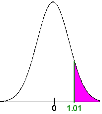
\[ Z = \dfrac{0-(-0.1)}{0.0995} = 1.01 \nonumber \]

Now we go to the table to find the associated probability. We get 0.8438. Since we want the area to the right, we subtract from 1 to get

\[ P(z > 1.01) = 1 - P(z < 1.01) = 1 - 0.8438 = 0.1562\nonumber \]

There is about a 16% chance that the gambler will not lose.

Distributions for Proportions

The last example was a special case of proportions, that is Boolean data. For now on, we can use the following theorem.

Central Limit Theory (for Proportions)

Let \(p\) be the probability of success, \(q\) be the probability of failure. The sampling distribution for samples of size \(n\) is approximately normal with mean

\[ \mu_{\overline{p}} = p \nonumber \]

and

\[ \sigma _ {\overline{p}} = \sqrt{\dfrac{pq}{n}} \nonumber \]

Example \(\PageIndex{3}\)

The new Endeavor SUV has been recalled because 5% of the cars experience brake failure. The Tahoe dealership has sold 200 of these cars. What is the probability that fewer than 4% of the cars from Tahoe experience brake failure?

Solution

We have \(p = 0.05 \), \(q = 0.95\) and \( n = 200\)

We have

\[ m_p = p = 0.05 \nonumber \]

\[\sigma_p = \sqrt{\dfrac{0.05 \cdot 0.95}{200}} = 0.0154 \nonumber \]

Next we want to find

\[ P(x < 8) \nonumber \]

Using the continuity correction, we find instead

\[ P(x < 7.5) \nonumber \]

This is equivalent to

\[ P(p < 7.5/200) = P(p < 0.0375) \nonumber \]

We find the z-score

0.0375 - 0.05
z = -0.81
0.0154

The table gives a probability of 0.2090. We can conclude that there is about a 21% chance that fewer than 4% of the cars will experience brake failure.

Charts for Proportions

For problems associated with proportions, we can use Control Charts and remembering that the Central Limit Theorem tells us how to find the mean and standard deviation.

Example 4

Heavenly Ski resort conducted a study of falls on its advanced run over twelve consecutive ten minute periods. At each ten minute interval there were 40 boarders on the run. The data is shown below:

Time	1	2	3	4	5	6	7	8	9	10	11	12
\(r\)	14	18	11	16	19	22	6	12	13	16	9	17
\(r/40\)	.35	0.45	0.275	.4	.475	.55	0.15	.3	0.325	0.4	0.225	0.425

Make a P-Chart and list any out of control signals by type (I, II, III).

Solution

First we find \(p\) by dividing the total number of falls by the total number of skiers:

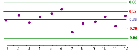
\[ p = \dfrac{173}{12(40)} = 0.36 \nonumber \]

Now we compute the mean

\[ \sigma = \sqrt{\dfrac{pq}{n}} = \sqrt{\dfrac{(0.36)(0.64)}{40}} = 0.08 \nonumber \]

Now we find two and three standard deviations above and below the mean are

\[ 0.36 - (2)(0.08) = 0.20 \nonumber \]

\[ 0.36 - (3)(0.08) = 0.04 \nonumber \]

\[ 0.36 + (2)(0.08) = 0.52 \nonumber \]

\[ 0.36 + (3)(0.08) = 0.68 \nonumber \]

Now we can use this data as before to construct a control chart and determine any out of control signals.

Notice that no nine consecutive points lie on one side of the blue line, no two of three points lie above 0.52 or below 0.20, and no points lie below 0.04 or above 0.68. Hence this data is in control.

Contributors and Attributions

• Contributors

  • Larry Green (Lake Tahoe Community College)