The Monte Carlo Simulation V2

What is a Monte Carlo Simulation?

A Monte Carlo technique describes any technique that uses random numbers and probability to solve a problem while a simulation is a numerical technique for conducting experiments on the computer. Putting the two terms together, Monte Carlo Simulation would then describe a class of computational algorithms that rely on repeated random sampling to obtain certain numerical results, and can be used to solve problems that have a probabilistic interpretation. Monte Carlo Simulation allows us to explicitly and quantitatively represent uncertainties. This means that simulation gives us insight on how likely our results are. Note that with any simulation, the results are as good as the inputs you give in. Poor inputs/model will lead to meaningless outputs.

Common tasks of the Monte Carlo Simulation include:

• Approximation of distribution of test statistics, estimators, etc.
• Approximation of quantities that allow for a probabilistic interpretation (in a certain sense). (E.g. Monte Carlo Integration, estimation of \( \pi \), etc)

For more examples of Monte Carlo in various fields, Wikipedia provides some good examples.

How does it work?

A typical Monte Carlo Simulation involves the following steps:

1. Define your inputs.
2. Model the system by using an appropriate probability density function.
3. Generate inputs randomly from the probability distribution.
4. Perform a deterministic computation on the inputs.
5. Repeat steps 2 and 3 as many times as desired.

Example 1 - Estimation of \( \pi \)

To estimate \( \pi \), we can imagine a circle enclosed by a square. We know that the area of the circle \( A_{circle} = \pi r^2 \) and the area of the square is \( A_{square} = 4r^2 \). Now, if we take a bunch of objects, say sand and splatter it onto the circle and square, the probability of the sand landing inside the circle will be \( P\){sand lands in circle} =\( \frac{\pi r^2}{4r^2} = \frac{\pi}{4} \). As a result, calculating \(\pi \) is a matter of calculating \(4 P\){sand lands in circle}. With our mathematical model defined, we can begin the Monte Carlo Simulation. First, we identify a probability density function that best models this phenomenon. The uniform distribution works well here because the probability of the sand landing in the square is equally likely. At the beginning of the simulation, initialize two variables, one to keep count of times we sample or drop a sand into the square and the second to count the number of sand that lands inside the circle. From the uniform distribution, we will sample for the location of the sand in the square; the \((x, y)\) coordinates. Next, we check whether the \((x, y)\) falls inside the circle using the formula \(x^2 + y^2 \leq r^2 \). To get the probability of sand inside the circle, we take the ratio of number of sand inside the circle over the number of sand we dropped onto the square.

#Simple R function to estimate pi. n is number of times to run the simulation and r is the radius of the circle. 

estimatePi = function(n, r)
{
  x = runif(n, -r, r)
  y = runif(n, -r, r)
  
  sum(x^2 + y^2 <= r^2)/n * 4
}

A great YouTube video explaining this example can be viewed here.

Example 2 - Approximating Distribution of Sample Mean

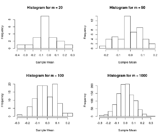
As a less rigorous application of the Monte Carlo Simulation in terms of statistics, we can try to approximate the distribution of the sample mean.

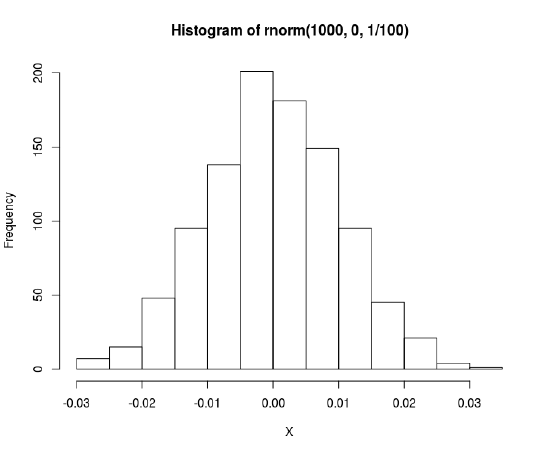
Sample mean is defined as \(\frac{1}{n}\sum_{i=1}^n X_{i}\). If we sample our data from \(N(0,1)\), then the distribution of the sample mean should be \(\bar{X} \sim N(0, \frac{1}{n} \)).

We can run a simulation in R to check this result.

#Number of times to repeat simulation
m = c(50,100,500,1000)

#Sample size
n = 100

generateSampleMeans = function(m) {
  replicate(m, {
  data = rnorm(n, 0, 1)
  sum(data)/sqrt(n)
  })
}

#Visualize histogram
par(mfrow=c(2,2)) 
sapply(m, function(i) 
  hist(generateSampleMeans(i), main = paste0("Histogram for m = ",i), xlab = "Sample Mean")

From the plot on the left, we can see that as number of iterations for the simulation increase, we get a histogram that looks more like the expected distribution for the sample mean as shown on the right.

Why does it work?

Convergence of the Monte Carlo Method means that you will get an approximately good estimation of your estimator. This convergence is implied by the law of large numbers. Specifically, it meets the requirement for the strong law of large numbers which in turn implies the weak law of large numbers. The intuition for the law of large numbers is that the Monte Carlo method requires repeated sampling and by law of large numbers, the average of the outcome you get will converge to the expected value. In the estimation of \( \pi \), we would expect that as we increase the amount of sand we drop onto the square, the closer we are to the value of \( \pi \).

Weak Law of Large Numbers:

Let \(X_{1}, X_{2}, . . .X_{n} \) be an i.i.d sequence of random variables for which \(\mathbf{E} X_{1} < \infty\). Then, \( \frac{1}{n} (X_{1} + . . . + X_{n}) \overset{P}{\rightarrow} \mathbf{E} [X_{1}] \ as \ n \rightarrow \infty \).

Strong Law of Large Numbers:

Suppose that the first moment of \( \mathbf{E} [(|X|)] \) is finite. Then \( \bar{ X_{n} } \) converges almost surely to \(\mathbf{E} [X]\), thus \(P(lim_{n -> \infty} \bar{ X_{n}} = \mathbf{E} [X]) = 1 \)

The law of large numbers guarantees convergence for the Monte Carlo Method, to identify the rate of convergence, it would require the central limit theorem. For a review of what the central limit theorem say, click here.

The central limit theorem tells us that the distribution of the errors will converge to a normal distribution and with this notion in mind, we can figure out the number of times we need to resample to achieve a certain accuracy. By assuming normal distribution of the errors, we have information to calculate the confidence interval and see what sample size is needed for the desired accuracy.

If we let \( \alpha_{n} \) be the numerical outcome we get and \(\alpha\) the expected estimator value we are trying to find, then by law of large numbers and central limit theorem, we can say that \(\alpha_{n} \overset{D}{\approx} \alpha + \frac{\sigma}{\sqrt{n}} N(0,1) \).

\( \overset{D}{\approx} \) denotes convergence in distribution. From this, we see that Monte Carlo converges very slowly because to achieve a tenfold accuracy, we would need to increase our sampling by a hundredfold.

References

Some resources that I used to write this page.

Stanford Lecture Notes - Quite detailed explanation.

Stack Exchange Question - Helped with the intuition behind why Monte Carlo converges.