4.1: Inferences about Two Means with Independent Samples (Assuming Unequal Variances)
- Page ID
- 2890
\( \newcommand{\vecs}[1]{\overset { \scriptstyle \rightharpoonup} {\mathbf{#1}} } \)
\( \newcommand{\vecd}[1]{\overset{-\!-\!\rightharpoonup}{\vphantom{a}\smash {#1}}} \)
\( \newcommand{\id}{\mathrm{id}}\) \( \newcommand{\Span}{\mathrm{span}}\)
( \newcommand{\kernel}{\mathrm{null}\,}\) \( \newcommand{\range}{\mathrm{range}\,}\)
\( \newcommand{\RealPart}{\mathrm{Re}}\) \( \newcommand{\ImaginaryPart}{\mathrm{Im}}\)
\( \newcommand{\Argument}{\mathrm{Arg}}\) \( \newcommand{\norm}[1]{\| #1 \|}\)
\( \newcommand{\inner}[2]{\langle #1, #2 \rangle}\)
\( \newcommand{\Span}{\mathrm{span}}\)
\( \newcommand{\id}{\mathrm{id}}\)
\( \newcommand{\Span}{\mathrm{span}}\)
\( \newcommand{\kernel}{\mathrm{null}\,}\)
\( \newcommand{\range}{\mathrm{range}\,}\)
\( \newcommand{\RealPart}{\mathrm{Re}}\)
\( \newcommand{\ImaginaryPart}{\mathrm{Im}}\)
\( \newcommand{\Argument}{\mathrm{Arg}}\)
\( \newcommand{\norm}[1]{\| #1 \|}\)
\( \newcommand{\inner}[2]{\langle #1, #2 \rangle}\)
\( \newcommand{\Span}{\mathrm{span}}\) \( \newcommand{\AA}{\unicode[.8,0]{x212B}}\)
\( \newcommand{\vectorA}[1]{\vec{#1}} % arrow\)
\( \newcommand{\vectorAt}[1]{\vec{\text{#1}}} % arrow\)
\( \newcommand{\vectorB}[1]{\overset { \scriptstyle \rightharpoonup} {\mathbf{#1}} } \)
\( \newcommand{\vectorC}[1]{\textbf{#1}} \)
\( \newcommand{\vectorD}[1]{\overrightarrow{#1}} \)
\( \newcommand{\vectorDt}[1]{\overrightarrow{\text{#1}}} \)
\( \newcommand{\vectE}[1]{\overset{-\!-\!\rightharpoonup}{\vphantom{a}\smash{\mathbf {#1}}}} \)
\( \newcommand{\vecs}[1]{\overset { \scriptstyle \rightharpoonup} {\mathbf{#1}} } \)
\( \newcommand{\vecd}[1]{\overset{-\!-\!\rightharpoonup}{\vphantom{a}\smash {#1}}} \)
\(\newcommand{\avec}{\mathbf a}\) \(\newcommand{\bvec}{\mathbf b}\) \(\newcommand{\cvec}{\mathbf c}\) \(\newcommand{\dvec}{\mathbf d}\) \(\newcommand{\dtil}{\widetilde{\mathbf d}}\) \(\newcommand{\evec}{\mathbf e}\) \(\newcommand{\fvec}{\mathbf f}\) \(\newcommand{\nvec}{\mathbf n}\) \(\newcommand{\pvec}{\mathbf p}\) \(\newcommand{\qvec}{\mathbf q}\) \(\newcommand{\svec}{\mathbf s}\) \(\newcommand{\tvec}{\mathbf t}\) \(\newcommand{\uvec}{\mathbf u}\) \(\newcommand{\vvec}{\mathbf v}\) \(\newcommand{\wvec}{\mathbf w}\) \(\newcommand{\xvec}{\mathbf x}\) \(\newcommand{\yvec}{\mathbf y}\) \(\newcommand{\zvec}{\mathbf z}\) \(\newcommand{\rvec}{\mathbf r}\) \(\newcommand{\mvec}{\mathbf m}\) \(\newcommand{\zerovec}{\mathbf 0}\) \(\newcommand{\onevec}{\mathbf 1}\) \(\newcommand{\real}{\mathbb R}\) \(\newcommand{\twovec}[2]{\left[\begin{array}{r}#1 \\ #2 \end{array}\right]}\) \(\newcommand{\ctwovec}[2]{\left[\begin{array}{c}#1 \\ #2 \end{array}\right]}\) \(\newcommand{\threevec}[3]{\left[\begin{array}{r}#1 \\ #2 \\ #3 \end{array}\right]}\) \(\newcommand{\cthreevec}[3]{\left[\begin{array}{c}#1 \\ #2 \\ #3 \end{array}\right]}\) \(\newcommand{\fourvec}[4]{\left[\begin{array}{r}#1 \\ #2 \\ #3 \\ #4 \end{array}\right]}\) \(\newcommand{\cfourvec}[4]{\left[\begin{array}{c}#1 \\ #2 \\ #3 \\ #4 \end{array}\right]}\) \(\newcommand{\fivevec}[5]{\left[\begin{array}{r}#1 \\ #2 \\ #3 \\ #4 \\ #5 \\ \end{array}\right]}\) \(\newcommand{\cfivevec}[5]{\left[\begin{array}{c}#1 \\ #2 \\ #3 \\ #4 \\ #5 \\ \end{array}\right]}\) \(\newcommand{\mattwo}[4]{\left[\begin{array}{rr}#1 \amp #2 \\ #3 \amp #4 \\ \end{array}\right]}\) \(\newcommand{\laspan}[1]{\text{Span}\{#1\}}\) \(\newcommand{\bcal}{\cal B}\) \(\newcommand{\ccal}{\cal C}\) \(\newcommand{\scal}{\cal S}\) \(\newcommand{\wcal}{\cal W}\) \(\newcommand{\ecal}{\cal E}\) \(\newcommand{\coords}[2]{\left\{#1\right\}_{#2}}\) \(\newcommand{\gray}[1]{\color{gray}{#1}}\) \(\newcommand{\lgray}[1]{\color{lightgray}{#1}}\) \(\newcommand{\rank}{\operatorname{rank}}\) \(\newcommand{\row}{\text{Row}}\) \(\newcommand{\col}{\text{Col}}\) \(\renewcommand{\row}{\text{Row}}\) \(\newcommand{\nul}{\text{Nul}}\) \(\newcommand{\var}{\text{Var}}\) \(\newcommand{\corr}{\text{corr}}\) \(\newcommand{\len}[1]{\left|#1\right|}\) \(\newcommand{\bbar}{\overline{\bvec}}\) \(\newcommand{\bhat}{\widehat{\bvec}}\) \(\newcommand{\bperp}{\bvec^\perp}\) \(\newcommand{\xhat}{\widehat{\xvec}}\) \(\newcommand{\vhat}{\widehat{\vvec}}\) \(\newcommand{\uhat}{\widehat{\uvec}}\) \(\newcommand{\what}{\widehat{\wvec}}\) \(\newcommand{\Sighat}{\widehat{\Sigma}}\) \(\newcommand{\lt}{<}\) \(\newcommand{\gt}{>}\) \(\newcommand{\amp}{&}\) \(\definecolor{fillinmathshade}{gray}{0.9}\)Up to this point, we have discussed inferences regarding a single population parameter (e.g., μ, p, \(\sigma^2\)). We have used sample data to construct confidence intervals to estimate the population mean or proportion and to test hypotheses about the population mean and proportion. In both of these chapters, all the examples involved the use of one sample to form an inference about one population. Frequently, we need to compare two sets of data, and make inferences about two populations. This chapter deals with inferences about two means, proportions, or variances. For example:
- You are studying turkey habitat and want to see if the mean number of brood hens is different in New York compared to Pennsylvania.
- You want to determine if the treatment used in Skaneateles Lake has reduced the number of milfoil plants over the last three years.
- Is the proportion of people who support alternative energy in California greater compared to New York?
- Is the variability in application different between two mist blowers?
These questions can be answered by comparing the differences of:
- Mean number of hens in NY to the mean number of hens in PA.
- Number of plants in 2007 to the number of plants in 2010.
- Proportion of people in CA to the proportion of people in NY.
- Variances between the mist blowers.
This chapter is comprised of five sections. The first and second sections examine inferences about two means with two independent samples. The third section examines inferences about means with two dependent samples, the fourth section examines inferences about two proportions, and the fifth section examines inferences between two variances.
Inferences about Two Means with Independent Samples (Assuming Unequal Variances)
Using independent samples means that there is no relationship between the groups. The values in one sample have no association with the values in the other sample. For example, we want to see if the mean life span for hummingbirds in South Carolina is different from the mean life span in North Carolina. These populations are not related, and the samples are independent. We look at the difference of the independent means.
In Chapter 3, we did a one-sample t-test where we compared the sample mean (\(\bar {x}\)) to the hypothesized mean (μ). We expect that \(\bar {x}\) would be close to μ. We use the sample mean, the sample standard deviation, and the sample size for the one-sample test.
With a two-sample t-test, we compare the population means to each other and again look at the difference. We expect that \(\bar {x_1}-\bar {x_2}\) would be close to \(\mu_{1} – \mu_{2}\). The test statistic will use both sample means, sample standard deviations, and sample sizes for the test.
- For a one-sample t-test we used \(\frac {s}{\sqrt{n}}\)as a measure of the standard deviation (the standard error).
- We can rewrite \(\frac {s}{\sqrt{n}} \rightarrow \sqrt {\frac {s^2}{n}}\)
- The numerator of the test statistic will be \((\bar {x_1} - \bar{x_2})-(\mu_{1} - \mu_{2})\)
- This has a standard deviation of \(\sqrt {\frac {s^2_1}{n_1}+\frac {s^2_2}{n_2}}\).
A two-sample t-test follows the same four steps we saw in Chapter 3.
- Write the null and alternative hypotheses.
- State the level of significance and find the critical value. The critical value, from the student’s t-distribution, has the lesser of n1-1 and n2 -1 degrees of freedom.
- Compute the test statistic.
- Compare the test statistic to the critical value and state a conclusion.
The assumptions we saw in Chapter 3 still must be met. Both samples come from independent random samples. The populations must be normally distributed, or both have large enough sample sizes (n1 and n2 ≥ 30). We will also use the same three pairs of null and alternative hypotheses.
Table \(\PageIndex{1}\). Null and alternative hypotheses.
| Two-sided | Left-sided | Right=sided |
| \(\mathrm{H}_{\mathrm{0}}: \mu_1=\mu_2\) | \(\mathrm{H}_{\mathrm{0}}: \mu_1=\mu_2\) | (\mathrm{H}_{\mathrm{0}}: \mu_1=\mu_2\) |
| \(\mathrm{H}_1: \mu_1 \neq \mu_2\) | \(\mathrm{H}_1: \mu_1<\mu_2\) | \(\mathrm{H}_1: \mu_1>\mu_2\) |
Rewriting the null hypothesis of μ1 = μ2 to μ1 – μ2 = 0, simplifies the numerator. The test statistic is Welch’s approximation (Satterthwaite Adjustment) under the assumption that the independent population variances are not equal.
\[t=\frac {(\bar {x_1}-\bar {x_2})-(\mu_{1}-\mu_{2})}{\sqrt {\frac {s^2_1}{n_1}+\frac {s^2_2}{n_2}}}\]
This test statistic follows the student’s t-distribution with the degrees of freedom adjusted by
\[df=\frac {(\frac {S^2_1}{n_1} + \frac {S^2_2}{n_2})^2}{\frac {1}{n_1-1}(\frac {S^2_1}{n_1})^2+\frac {1}{n_2-1}(\frac {S^2_2}{n_2})^2}\]
A simpler alternative to determining degrees of freedom when working a problem long-hand is to use the lesser of n1-1 or n2-1 as the degrees of freedom. This method results in a smaller value for degrees of freedom and therefore a larger critical value. This makes the test more conservative, requiring more evidence to reject the null hypothesis.
A forester is studying the number of cavity trees in old growth stands in Adirondack Park in northern New York. He wants to know if there is a significant difference between the mean number of cavity trees in the Adirondack Park and the old growth stands in the Monongahela National Forest. He collects two independent random samples from each forest. Use a 5% level of significance to test this claim.
|
Adirondack Park |
Monongahela Forest |
|
\(n_1\) = 51 stands |
\(n_2\) = 56 stands |
|
\(\bar {x_1}\)= 39.6 |
\(\bar {x_2}\)= 43.9 |
|
\(s_1\) = 9.4 |
\(s_2\) = 10.7 |
1) \(H_0: \mu_1 = \mu_2 or \mu_1 – \mu_2 = 0\) There is no difference between the two population means.
\(H_1: \mu_1 ≠ \mu_2\) There is a difference between the two population means.
2) The level of significance is 5%. This is a two-sided test so alpha is split into two sides. Computing degrees of freedom using the equation above gives 105 degrees of freedom.
\[df = \frac {(\frac {9.4^2}{51}+\frac {10.7^2}{56})^2}{\frac {1}{51-1}(\frac {9.4^2}{51})^2+\frac {1}{56-1}(\frac {10.7^2}{56})^2}=104.9 \nonumber \]
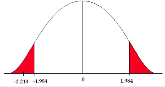
The critical value (\(t_{\frac {\alpha}{2}}\), based on 100 degrees of freedom (closest value in the t-table), is ±1.984. Using 50 degrees of freedom, the critical value is ±2.009.
3) The test statistic is
\[t=\frac {(\bar {x_1} - \bar {x_2}) - (\mu _1 - \mu_2)}{\sqrt {\frac {s_1^2}{n_1}+\frac {s_2^2}{n_2}}} =\frac {(39.6-43.9)-(0)}{\sqrt{\frac {9.4^2}{51}+\frac {10.7^2}{56}}} = -2.213 \nonumber\]
4) The test statistic falls in the rejection zone.

We reject the null hypothesis. We have enough evidence to support the claim that there is a difference in the mean number of cavity trees between the Adirondack Park and the Monongahela National Forest.
Construct and Interpret a Confidence Interval about the Difference of Two Independent Means
A hypothesis test will answer the question about the difference of the means. BUT, we can answer the same question by constructing a confidence interval about the difference of the means. This process is just like the confidence intervals from Chapter 2.
- Find the critical value.
- Compute the margin of error.
- Point estimate ± margin of error.
Because we are working with two samples, we must modify the components of the confidence interval to incorporate the information from the two populations.
- The point estimate is \(\bar {x_1} -\bar {x_2}\).
- The standard error comes from the test statistic \(\sqrt {\frac {s_1^2}{n_1} +\frac {s^2_2}{n_2}}\)
- The critical value \(t_{\frac {\alpha}{2}}\)comes from the student’s t-table.
The confidence interval takes the form of the point estimate plus or minus the standard error of the differences.
\[\bar {x_1} -\bar {x_2} \pm t_{\frac {\alpha}{2}}\sqrt {\frac {s_1^2}{n_1} +\frac {s^2_2}{n_2}}\]
We will use the same three steps to construct a confidence interval about the difference of the means.
- critical value \(t_{\frac {\alpha}{2}}\)
- \(E = t_{\frac {\alpha}{2}}\sqrt {\frac {s_1^2}{n_1} +\frac {s^2_2}{n_2}}\)
- \(\bar {x_1} -\bar {x_2} \pm E\)
Let’s look at the mean number of cavity trees in old growth stands again. The forester wants to know if there is a difference between the mean number of cavity trees in old growth stands in the Adirondack forests and in the Monongahela Forest. We can answer this question by constructing a confidence interval about the difference of the means.
1) \(t_{\frac {\alpha}{2}}\) = 2.009
2) \(E = t_{\frac {\alpha}{2}}\sqrt {\frac {s_1^2}{n_1} +\frac {s^2_2}{n_2}} = 2.009 \sqrt {\frac {9.4^2}{51}+\frac {10.7^2}{56}}=3.904\)
3) \(\bar {x_1} -\bar {x_2} \pm 3.904\)
The 95% confidence interval for the difference of the means is (-8.204, -0.396).
We can be 95% confident that this interval contains the mean difference in number of cavity trees between the two locations. BUT, this doesn’t answer the question the forester asked. Is there a difference in the mean number of cavity trees between the Adirondack and Monongahela forests? To answer this, we must look at the confidence interval interpretations.
Confidence Interval Interpretations
- If the confidence interval contains all positive values, we find a significant difference between the groups, AND we can conclude that the mean of the first group is significantly greater than the mean of the second group.
- If the confidence interval contains all negative values, we find a significant difference between the groups, AND we can conclude that the mean of the first group is significantly less than the mean of the second group.
- If the confidence interval contains zero (it goes from negative to positive values), we find NO significant difference between the groups.
In this problem, the confidence interval is (-8.204, -0.396). We have all negative values, so we can conclude that there is a significant difference in the mean number of cavity trees AND that the mean number of cavity trees in the Adirondack forests is significantly less than the mean number of cavity trees in the Monongahela Forest. The confidence interval gives an estimate of the mean difference in number of cavity trees between the two forests. There are, on average, 0.396 to 8.204 fewer cavity trees in the Adirondack Park than the Monongahela Forest.
P-value Approach
We can also use the p-value approach to answer the question. Remember, the p-value is the area under the normal curve associated with the test statistic. This example is a two-sided test (H1: μ1 ≠ μ2 ) so the p-value, when computed by hand, will be multiplied by two.
The test statistic equals -2.213, so the p-value is two times the area to the left of -2.213. We can only estimate the p-value using the student’s t-table. Using the lesser of n1– 1 or n2– 1 as the degrees of freedom, we have 50 degrees of freedom. Go across the 50 row in the student’s t-table until you find the absolute value of the test statistic. In this case, 2.213 falls between 2.109 and 2.403. Going up to the top of each of those columns gives you the estimate of the p-value (between 0.02 and 0.01).
Table \(\PageIndex{2}\). Student t-Distribution Area in Right Tail
|
df |
.05 |
.025 |
.02 |
.01 |
.005 |
|---|---|---|---|---|---|
|
39 |
1.686 |
2.024 |
2.127 |
2.429 |
2.712 |
|
40 |
1.684 |
2.021 |
2.123 |
2.423 |
2.704 |
|
50 |
1.676 |
2.009 |
2.109 |
2.403 |
2.678 |
|
60 |
1.671 |
2.000 |
2.099 |
2.390 |
2.660 |
|
70 |
1.667 |
1.994 |
2.093 |
2.381 |
2.648 |
The p-value is 2x(0.01 – 0.02) = (0.02 < p < 0.04). The p-value is greater than 0.02 but less than 0.04. This is less than the level of significance (0.05), so we reject the null hypothesis. There is enough evidence to support the claim that there is a significant difference in the mean number of cavity trees between the areas.
Researchers are studying the relationship between logging activities in the northern forests and amphibian habitats. They were comparing moisture levels between old-growth and post-harvest habitats. The researchers believe that post-harvest habitat has a lower moisture level. They collected data on moisture levels from two independent random samples. Test their claim using a 5% level of significance.
|
Old Growth |
Post Harvest |
|---|---|
|
n1 = 26 |
n2 = 31 |
|
|
|
|
s1 = 0.12 g/cm3 |
s2 = 0.17 g/cm3 |
H0: μ1 = μ2 or μ1 – μ2 = 0. There is no difference between the two population means.
H1: μ1 > μ2. Mean moisture level in old growth forests is greater than post-harvest levels.
We will use the critical value based on the lesser of n1– 1 or n2– 1 degrees of freedom. In this problem, there are 25 degrees of freedom and the critical value is 1.708. Now compute the test statistic.
\[t=\frac {(0.62-0.56)-0}{\sqrt {\frac {0.12^2}{26}+\frac {0.17^2}{31}}} = 1.556\]
The test statistic does not fall in the rejection zone. We fail to reject the null hypothesis. There is not enough evidence to support the claim that the moisture level is significantly lower in the post-harvest habitat.
Now answer this question by constructing a 90% confidence interval about the difference of the means.
1) \(t_{\frac {\alpha}{2}}\) = 1.708
2) E = \(t_{\frac {\alpha}{2}}\)\(\sqrt {\frac {s_1^2}{n_1}+\frac {s^2_2}{n_2}}=1.708\sqrt {\frac {0.12^2}{26}+\frac {0.17^2}{31}}=0.0658\)
3) \(\bar {x_1} -\bar {x_2} \pm E= (0.62-0.56) ±0.0658\)
The 90% confidence interval for the difference of the means is (-0.0058, 0.1258). The values in the confidence interval run from negative to positive indicating that there is no significant different in the mean moisture levels between old growth and post-harvest stands.
Software Solutions
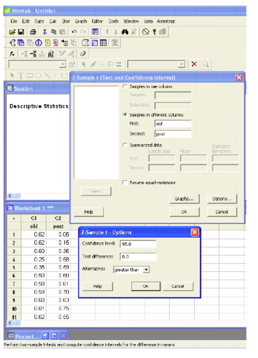
Minitab


Two-Sample T-Test and CI: for old vs. post
|
N |
Mean |
StDev |
SE Mean |
|
|---|---|---|---|---|
|
old |
26 |
0.620 |
0.121 |
0.024 |
|
post |
31 |
0.559 |
0.172 |
0.031 |
|
Difference = \(\mu_{(old)} – \mu_{(post)}\) |
||||
|
Estimate for difference: 0.0603 |
||||
|
95% lower bound for difference: -0.0049 |
||||
|
T-Test of difference = 0 (vs >): T-Value = 1.55 p-Value = 0.064 DF = 53 |
||||
The p-value (0.064) is greater than the level of confidence so we fail to reject the null hypothesis.
Additional example: www.youtube.com/watch?v=7pIb-GVixFo.
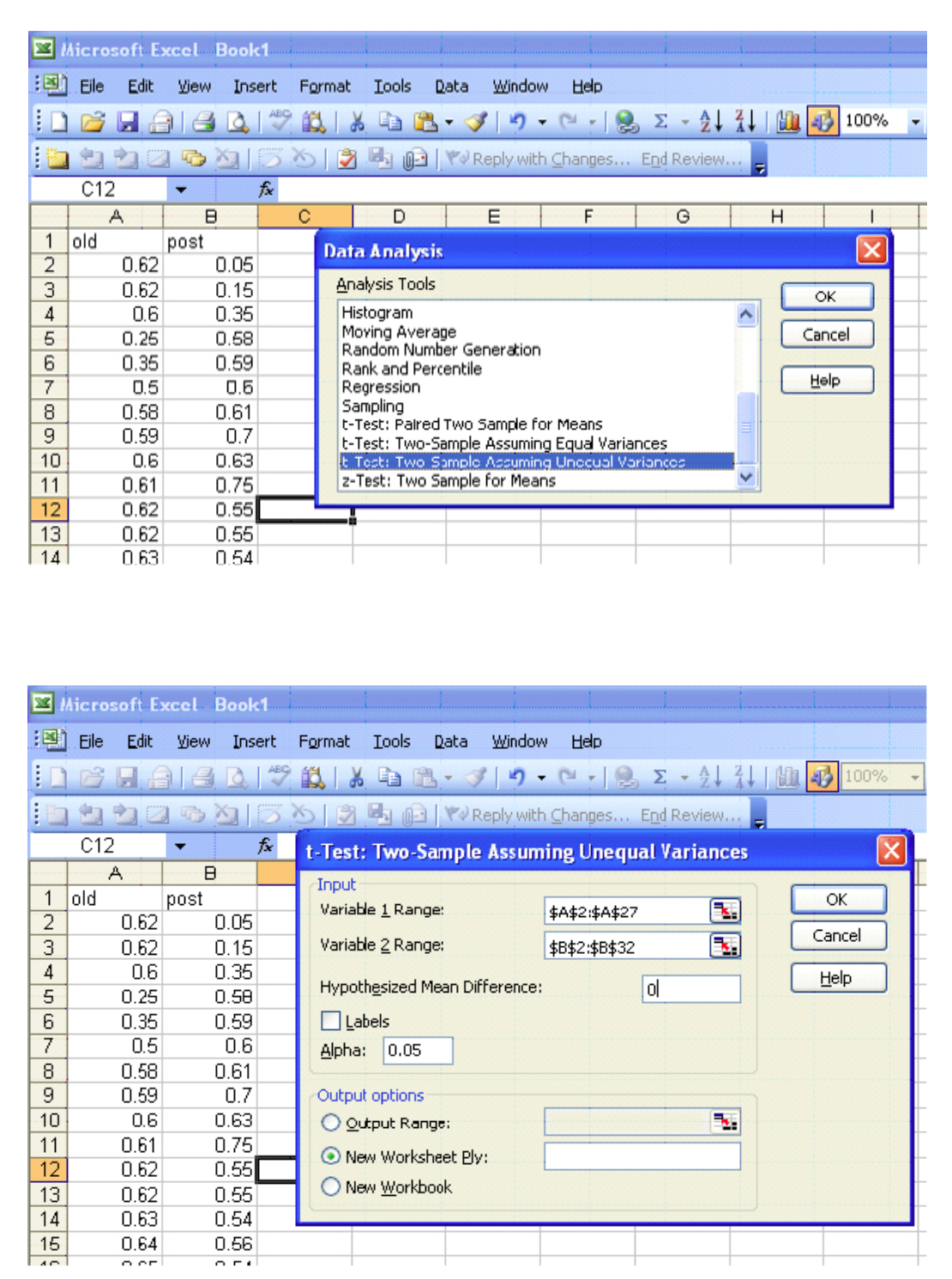
Excel

t-Test: Two-Sample Assuming Unequal Variances
|
Variable 1 |
Variable 2 |
|
|---|---|---|
|
Mean |
0.619615 |
0.559355 |
|
Variance |
0.014708 |
0.02948 |
|
Observations |
26 |
31 |
|
Hypothesized Mean Difference |
0 |
|
|
df |
54 |
|
|
t Stat |
1.557361 |
|
|
\(P(T\le t)\) one-tail |
0.063809 |
|
|
t Critical one-tail |
1.673565 |
|
|
\(P(T\le t)\) two-tail |
0.127617 |
|
|
t Critical two-tail |
2.004879 |
The one-tail p-value (0.063809) is greater than the level of significance, therefore, we fail to reject the null hypothesis.


 =0.62 g/cm3
 = 0.56 g/cm3