A.8: Use R in the cloud
- Page ID
- 45303
\( \newcommand{\vecs}[1]{\overset { \scriptstyle \rightharpoonup} {\mathbf{#1}} } \)
\( \newcommand{\vecd}[1]{\overset{-\!-\!\rightharpoonup}{\vphantom{a}\smash {#1}}} \)
\( \newcommand{\dsum}{\displaystyle\sum\limits} \)
\( \newcommand{\dint}{\displaystyle\int\limits} \)
\( \newcommand{\dlim}{\displaystyle\lim\limits} \)
\( \newcommand{\id}{\mathrm{id}}\) \( \newcommand{\Span}{\mathrm{span}}\)
( \newcommand{\kernel}{\mathrm{null}\,}\) \( \newcommand{\range}{\mathrm{range}\,}\)
\( \newcommand{\RealPart}{\mathrm{Re}}\) \( \newcommand{\ImaginaryPart}{\mathrm{Im}}\)
\( \newcommand{\Argument}{\mathrm{Arg}}\) \( \newcommand{\norm}[1]{\| #1 \|}\)
\( \newcommand{\inner}[2]{\langle #1, #2 \rangle}\)
\( \newcommand{\Span}{\mathrm{span}}\)
\( \newcommand{\id}{\mathrm{id}}\)
\( \newcommand{\Span}{\mathrm{span}}\)
\( \newcommand{\kernel}{\mathrm{null}\,}\)
\( \newcommand{\range}{\mathrm{range}\,}\)
\( \newcommand{\RealPart}{\mathrm{Re}}\)
\( \newcommand{\ImaginaryPart}{\mathrm{Im}}\)
\( \newcommand{\Argument}{\mathrm{Arg}}\)
\( \newcommand{\norm}[1]{\| #1 \|}\)
\( \newcommand{\inner}[2]{\langle #1, #2 \rangle}\)
\( \newcommand{\Span}{\mathrm{span}}\) \( \newcommand{\AA}{\unicode[.8,0]{x212B}}\)
\( \newcommand{\vectorA}[1]{\vec{#1}} % arrow\)
\( \newcommand{\vectorAt}[1]{\vec{\text{#1}}} % arrow\)
\( \newcommand{\vectorB}[1]{\overset { \scriptstyle \rightharpoonup} {\mathbf{#1}} } \)
\( \newcommand{\vectorC}[1]{\textbf{#1}} \)
\( \newcommand{\vectorD}[1]{\overrightarrow{#1}} \)
\( \newcommand{\vectorDt}[1]{\overrightarrow{\text{#1}}} \)
\( \newcommand{\vectE}[1]{\overset{-\!-\!\rightharpoonup}{\vphantom{a}\smash{\mathbf {#1}}}} \)
\( \newcommand{\vecs}[1]{\overset { \scriptstyle \rightharpoonup} {\mathbf{#1}} } \)
\(\newcommand{\longvect}{\overrightarrow}\)
\( \newcommand{\vecd}[1]{\overset{-\!-\!\rightharpoonup}{\vphantom{a}\smash {#1}}} \)
\(\newcommand{\avec}{\mathbf a}\) \(\newcommand{\bvec}{\mathbf b}\) \(\newcommand{\cvec}{\mathbf c}\) \(\newcommand{\dvec}{\mathbf d}\) \(\newcommand{\dtil}{\widetilde{\mathbf d}}\) \(\newcommand{\evec}{\mathbf e}\) \(\newcommand{\fvec}{\mathbf f}\) \(\newcommand{\nvec}{\mathbf n}\) \(\newcommand{\pvec}{\mathbf p}\) \(\newcommand{\qvec}{\mathbf q}\) \(\newcommand{\svec}{\mathbf s}\) \(\newcommand{\tvec}{\mathbf t}\) \(\newcommand{\uvec}{\mathbf u}\) \(\newcommand{\vvec}{\mathbf v}\) \(\newcommand{\wvec}{\mathbf w}\) \(\newcommand{\xvec}{\mathbf x}\) \(\newcommand{\yvec}{\mathbf y}\) \(\newcommand{\zvec}{\mathbf z}\) \(\newcommand{\rvec}{\mathbf r}\) \(\newcommand{\mvec}{\mathbf m}\) \(\newcommand{\zerovec}{\mathbf 0}\) \(\newcommand{\onevec}{\mathbf 1}\) \(\newcommand{\real}{\mathbb R}\) \(\newcommand{\twovec}[2]{\left[\begin{array}{r}#1 \\ #2 \end{array}\right]}\) \(\newcommand{\ctwovec}[2]{\left[\begin{array}{c}#1 \\ #2 \end{array}\right]}\) \(\newcommand{\threevec}[3]{\left[\begin{array}{r}#1 \\ #2 \\ #3 \end{array}\right]}\) \(\newcommand{\cthreevec}[3]{\left[\begin{array}{c}#1 \\ #2 \\ #3 \end{array}\right]}\) \(\newcommand{\fourvec}[4]{\left[\begin{array}{r}#1 \\ #2 \\ #3 \\ #4 \end{array}\right]}\) \(\newcommand{\cfourvec}[4]{\left[\begin{array}{c}#1 \\ #2 \\ #3 \\ #4 \end{array}\right]}\) \(\newcommand{\fivevec}[5]{\left[\begin{array}{r}#1 \\ #2 \\ #3 \\ #4 \\ #5 \\ \end{array}\right]}\) \(\newcommand{\cfivevec}[5]{\left[\begin{array}{c}#1 \\ #2 \\ #3 \\ #4 \\ #5 \\ \end{array}\right]}\) \(\newcommand{\mattwo}[4]{\left[\begin{array}{rr}#1 \amp #2 \\ #3 \amp #4 \\ \end{array}\right]}\) \(\newcommand{\laspan}[1]{\text{Span}\{#1\}}\) \(\newcommand{\bcal}{\cal B}\) \(\newcommand{\ccal}{\cal C}\) \(\newcommand{\scal}{\cal S}\) \(\newcommand{\wcal}{\cal W}\) \(\newcommand{\ecal}{\cal E}\) \(\newcommand{\coords}[2]{\left\{#1\right\}_{#2}}\) \(\newcommand{\gray}[1]{\color{gray}{#1}}\) \(\newcommand{\lgray}[1]{\color{lightgray}{#1}}\) \(\newcommand{\rank}{\operatorname{rank}}\) \(\newcommand{\row}{\text{Row}}\) \(\newcommand{\col}{\text{Col}}\) \(\renewcommand{\row}{\text{Row}}\) \(\newcommand{\nul}{\text{Nul}}\) \(\newcommand{\var}{\text{Var}}\) \(\newcommand{\corr}{\text{corr}}\) \(\newcommand{\len}[1]{\left|#1\right|}\) \(\newcommand{\bbar}{\overline{\bvec}}\) \(\newcommand{\bhat}{\widehat{\bvec}}\) \(\newcommand{\bperp}{\bvec^\perp}\) \(\newcommand{\xhat}{\widehat{\xvec}}\) \(\newcommand{\vhat}{\widehat{\vvec}}\) \(\newcommand{\uhat}{\widehat{\uvec}}\) \(\newcommand{\what}{\widehat{\wvec}}\) \(\newcommand{\Sighat}{\widehat{\Sigma}}\) \(\newcommand{\lt}{<}\) \(\newcommand{\gt}{>}\) \(\newcommand{\amp}{&}\) \(\definecolor{fillinmathshade}{gray}{0.9}\)A quick guide about how to how to run R via a cloud computing (serverless) option.
Installation guides quickly become outdated. This page was last updated 19 August 2024 and describes working installation protocols at that time.
Run R on your computer (i.e., local development environment or LDE)
This guide is about running R in the cloud, serverless options. For installing R and R Commander onto your own computer, see Install R and Install R Commander.
Run R “in the Cloud”
If you do not wish to install R, or if you have a ARM-based Chromebook and therefore cannot gracefully install R, then there are alternatives: Run R in the Cloud. I’ll list five ways to run R in the cloud — run R on a server, not your own computer — for free.
Note: None of these options can run R Commander, which requires a local (on your computer) installation of R.
If you have a Chromebook, or you want to run R on your tablet (iPad, Kindle, etc.), you can’t install R to any of these devices. However, you can access R via a serverless Cloud solution.
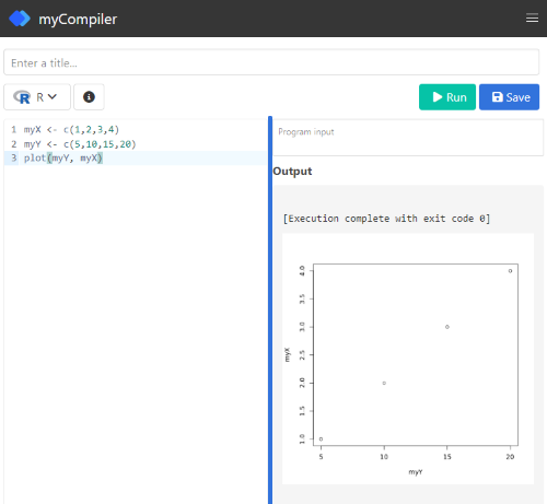
1. Run R code at Online R Compiler using myCompiler’s online IDE, link at https://www.mycompiler.io/online-r-compiler.

2. Run code snippets in CoCalc by folks at SageMath and available at https://cocalc.com/. CoCalc uses Jupyter Notebooks, a wonderful, open-source project which supports interactive computer coding for many languages, including R and Markdown.
While CoLab is my go to, CoCalc is a really good student option — hint: I have my Systems Biology students use this option — includes SageMATH, python, GNU Octave and other software.
Create a free account (you’ll then be able to save your code), or simply click “Run CoCalc Now” and check the box to agree to the terms to begin a session (Fig. \(\PageIndex{2}\)). Choose to open a new Jupyter notebook, then select R (system wide) from the choice of kernels.

You can load files from your computer for use in CoCalc sessions. There is also a version of the software you can download to your computer.
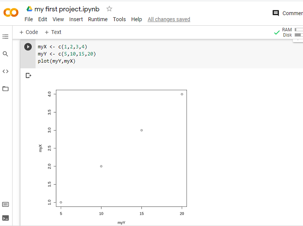
3. My favorite option, run R code snippets at Google Colaboratory (Fig. \(\PageIndex{3}\)). Like CoCalc, Colaboratory uses Jupyter Notebooks. Log into your Google account, then click https://colab.research.google.com/notebook#create=true&language=r , or try the tinyURL https://colab.to/r

Colabs is worth the effort — you end up with a system to run R in your browser, it’s free to use, and you can store/retrieve files from your Google Drive. This is my choice for Cloud computing, and it’s the most generic solution. For more information, see post by Ed Adityawarman, How to use R in Google Colab . Colab Jupyter notebooks use Python by default. To run R, either use the link listed above each time you want to create a new R notebook, or add the following code snippet to your new notebook page
# activate R magic - must begin each R code with %%R
%load_ext rpy2.ipython
For all subsequent R code, start the section with
%%R
Note: You can install Jupyter onto your computer via Miniconda — conda is an open source package management system but then, you still would have to install R to your computer.
One real advantage of choosing CoLab, there are apps to run Google Colaboratory and Jupyter Notebooks on iPad/iPhone and for Android phones are available at Apple App Store and Google Play, respectively.
4. You can run RStudio at Posit Cloud. Registration and use is free for students. This works OK, but can be slow and it’s hard to work on your own data. It does have the advantage of providing the familiar RStudio interface. Choose the free plan; Instructions to get started are at https://posit.cloud/plans. A screenshot of an RStudio cloud session is shown in Figure \(\PageIndex{4}\).

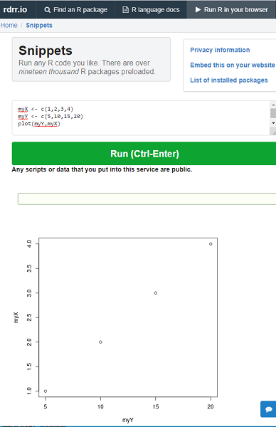
5. For limited use, i.e., you just need to run a little code to solve an assignment problem, you can run R code snippets in your browser at https://rdrr.io/snippets/ . You’ll see many of my code embedded in this service so that you can run code snippets from my Chaminade University CANVAS pages.


