
16.6: Similarity and distance
- Page ID
- 45246

\( \newcommand{\vecs}[1]{\overset { \scriptstyle \rightharpoonup} {\mathbf{#1}} } \)
\( \newcommand{\vecd}[1]{\overset{-\!-\!\rightharpoonup}{\vphantom{a}\smash {#1}}} \)
\( \newcommand{\id}{\mathrm{id}}\) \( \newcommand{\Span}{\mathrm{span}}\)
( \newcommand{\kernel}{\mathrm{null}\,}\) \( \newcommand{\range}{\mathrm{range}\,}\)
\( \newcommand{\RealPart}{\mathrm{Re}}\) \( \newcommand{\ImaginaryPart}{\mathrm{Im}}\)
\( \newcommand{\Argument}{\mathrm{Arg}}\) \( \newcommand{\norm}[1]{\| #1 \|}\)
\( \newcommand{\inner}[2]{\langle #1, #2 \rangle}\)
\( \newcommand{\Span}{\mathrm{span}}\)
\( \newcommand{\id}{\mathrm{id}}\)
\( \newcommand{\Span}{\mathrm{span}}\)
\( \newcommand{\kernel}{\mathrm{null}\,}\)
\( \newcommand{\range}{\mathrm{range}\,}\)
\( \newcommand{\RealPart}{\mathrm{Re}}\)
\( \newcommand{\ImaginaryPart}{\mathrm{Im}}\)
\( \newcommand{\Argument}{\mathrm{Arg}}\)
\( \newcommand{\norm}[1]{\| #1 \|}\)
\( \newcommand{\inner}[2]{\langle #1, #2 \rangle}\)
\( \newcommand{\Span}{\mathrm{span}}\) \( \newcommand{\AA}{\unicode[.8,0]{x212B}}\)
\( \newcommand{\vectorA}[1]{\vec{#1}} % arrow\)
\( \newcommand{\vectorAt}[1]{\vec{\text{#1}}} % arrow\)
\( \newcommand{\vectorB}[1]{\overset { \scriptstyle \rightharpoonup} {\mathbf{#1}} } \)
\( \newcommand{\vectorC}[1]{\textbf{#1}} \)
\( \newcommand{\vectorD}[1]{\overrightarrow{#1}} \)
\( \newcommand{\vectorDt}[1]{\overrightarrow{\text{#1}}} \)
\( \newcommand{\vectE}[1]{\overset{-\!-\!\rightharpoonup}{\vphantom{a}\smash{\mathbf {#1}}}} \)
\( \newcommand{\vecs}[1]{\overset { \scriptstyle \rightharpoonup} {\mathbf{#1}} } \)
\( \newcommand{\vecd}[1]{\overset{-\!-\!\rightharpoonup}{\vphantom{a}\smash {#1}}} \)
\(\newcommand{\avec}{\mathbf a}\) \(\newcommand{\bvec}{\mathbf b}\) \(\newcommand{\cvec}{\mathbf c}\) \(\newcommand{\dvec}{\mathbf d}\) \(\newcommand{\dtil}{\widetilde{\mathbf d}}\) \(\newcommand{\evec}{\mathbf e}\) \(\newcommand{\fvec}{\mathbf f}\) \(\newcommand{\nvec}{\mathbf n}\) \(\newcommand{\pvec}{\mathbf p}\) \(\newcommand{\qvec}{\mathbf q}\) \(\newcommand{\svec}{\mathbf s}\) \(\newcommand{\tvec}{\mathbf t}\) \(\newcommand{\uvec}{\mathbf u}\) \(\newcommand{\vvec}{\mathbf v}\) \(\newcommand{\wvec}{\mathbf w}\) \(\newcommand{\xvec}{\mathbf x}\) \(\newcommand{\yvec}{\mathbf y}\) \(\newcommand{\zvec}{\mathbf z}\) \(\newcommand{\rvec}{\mathbf r}\) \(\newcommand{\mvec}{\mathbf m}\) \(\newcommand{\zerovec}{\mathbf 0}\) \(\newcommand{\onevec}{\mathbf 1}\) \(\newcommand{\real}{\mathbb R}\) \(\newcommand{\twovec}[2]{\left[\begin{array}{r}#1 \\ #2 \end{array}\right]}\) \(\newcommand{\ctwovec}[2]{\left[\begin{array}{c}#1 \\ #2 \end{array}\right]}\) \(\newcommand{\threevec}[3]{\left[\begin{array}{r}#1 \\ #2 \\ #3 \end{array}\right]}\) \(\newcommand{\cthreevec}[3]{\left[\begin{array}{c}#1 \\ #2 \\ #3 \end{array}\right]}\) \(\newcommand{\fourvec}[4]{\left[\begin{array}{r}#1 \\ #2 \\ #3 \\ #4 \end{array}\right]}\) \(\newcommand{\cfourvec}[4]{\left[\begin{array}{c}#1 \\ #2 \\ #3 \\ #4 \end{array}\right]}\) \(\newcommand{\fivevec}[5]{\left[\begin{array}{r}#1 \\ #2 \\ #3 \\ #4 \\ #5 \\ \end{array}\right]}\) \(\newcommand{\cfivevec}[5]{\left[\begin{array}{c}#1 \\ #2 \\ #3 \\ #4 \\ #5 \\ \end{array}\right]}\) \(\newcommand{\mattwo}[4]{\left[\begin{array}{rr}#1 \amp #2 \\ #3 \amp #4 \\ \end{array}\right]}\) \(\newcommand{\laspan}[1]{\text{Span}\{#1\}}\) \(\newcommand{\bcal}{\cal B}\) \(\newcommand{\ccal}{\cal C}\) \(\newcommand{\scal}{\cal S}\) \(\newcommand{\wcal}{\cal W}\) \(\newcommand{\ecal}{\cal E}\) \(\newcommand{\coords}[2]{\left\{#1\right\}_{#2}}\) \(\newcommand{\gray}[1]{\color{gray}{#1}}\) \(\newcommand{\lgray}[1]{\color{lightgray}{#1}}\) \(\newcommand{\rank}{\operatorname{rank}}\) \(\newcommand{\row}{\text{Row}}\) \(\newcommand{\col}{\text{Col}}\) \(\renewcommand{\row}{\text{Row}}\) \(\newcommand{\nul}{\text{Nul}}\) \(\newcommand{\var}{\text{Var}}\) \(\newcommand{\corr}{\text{corr}}\) \(\newcommand{\len}[1]{\left|#1\right|}\) \(\newcommand{\bbar}{\overline{\bvec}}\) \(\newcommand{\bhat}{\widehat{\bvec}}\) \(\newcommand{\bperp}{\bvec^\perp}\) \(\newcommand{\xhat}{\widehat{\xvec}}\) \(\newcommand{\vhat}{\widehat{\vvec}}\) \(\newcommand{\uhat}{\widehat{\uvec}}\) \(\newcommand{\what}{\widehat{\wvec}}\) \(\newcommand{\Sighat}{\widehat{\Sigma}}\) \(\newcommand{\lt}{<}\) \(\newcommand{\gt}{>}\) \(\newcommand{\amp}{&}\) \(\definecolor{fillinmathshade}{gray}{0.9}\)Introduction
A measure of dependence between two random variables. Unlike Pearson Product Moment correlation, distance correlation measures strength of association between the variables whether or not the relationship is linear. Distance correlation is a recent addition to the literature, first reported by Gábor J. Székely (e.g., Székely et al. 2007). The package correlation (Makowski et al 2019) offers distance correlation and significance test.
Example, fly wing dataset introduced 16.1 – Product moment correlation
library(correlation)
Area <- c(0.446, 0.876, 0.390, 0.510, 0.736, 0.453, 0.882, 0.394, 0.503, 0.535, 0.441, 0.889, 0.391, 0.514, 0.546, 0.453, 0.882, 0.394, 0.503, 0.535)
Length <- c(1.524, 2.202, 1.520, 1.620, 1.710, 1.551, 2.228, 1.460, 1.659, 1.719, 1.534, 2.223, 1.490, 1.633, 1.704, 1.551, 2.228, 1.468, 1.659, 1.719)
FlyWings <- data.frame(Area, Length)
correlation(FlyWings,method="distance")
Output from R
# Correlation Matrix (distance-method)
Parameter1 | Parameter2 |    r |       95% CI | t(169) |      p
------------------------------------------------------------------
      Area |     Length | 0.92 | [0.80, 0.97] |  30.47 | < .001***

p-value adjustment method: Holm (1979)
Observations: 20
The product-moment correlation was 0.97 with 95% confidence interval (0.92, 0.99). The note about “p-value adjustment method: Holm (1979)” refers to the algorithm used to mitigate the multicomparison problem, which we first introduced in Chapter 12.1. The correction is necessary in this context because of how the algorithm conducts the test of the distance correlation. Please see Székely and Rizzo (2013) for more details.
Which should you report? For cases where it makes sense to test for a linear association, then the product-moment correlation is the one to use. For other cases where no inference of linearity is expected, then the distance correlation makes sense.
Similarity and Distance
Similarity and distance are related mathematically. When two things are similar, the distance between them is small; When two things are dissimilar, the distance between them is great. Whether similarity (sometimes dissimilarity) or distance, the estimate is a statistic. The difference between the two is that the typical distance measures one sees in biostatistics all obey the triangle inequality rule while similarity (dissimilarity) indices do not necessarily obey the triangle inequality rule.
Distance measures
Distance is a way to talk about how far (or how close) two objects are from each other (Fig. \(\PageIndex{1}\)). The distance may be relate to physical distance (map distance), or in mathematics, distance is a metric or statistic. Euclidean distance is the distance between two points in either the \(xy\)-plane or 3-dimensional space measures the length of a segment connecting the two points (e.g., \(x_{1}, y_{1} = 1, 4\) and \(x_{2}, y_{2} = 1,4\)).
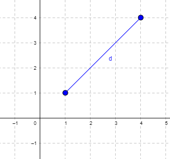
For two points \((x_{1}, y_{1}\) and \(x_{2}, y_{2}\)) described in two dimensions (e.g., an \(xy\)-plane), the distance \(d\) is given by \[d = \sqrt{\left(x_{1} - x_{2}\right)^{2} - \left(y_{1} - y_{2}\right)^{2}} \nonumber\]
For two points described in three (e.g., an \(xyz\)-space), or more dimensions, the distance \(d\) is given by \[d = \sqrt{\sum_{i=1}^{n} \left(x_{i} - y_{i}\right)^{2}} \nonumber\]
Distances of this form are Euclidean distances and can be directly obtained by use of the Pythagorean Theorem. The triangle inequality rule then applies (i.e., the sum of any two sides must be less than the length of the remaining side). Euclidean distance measures also include
- Manhattan distance: the sum of absolute difference between the measures in all dimensions of two points.
\(\left|x_{1} - x_{2}\right| + \left|y_{1} - y_{2}\right|\)
- Chebyshev distance: also called the maximum value distance, the distance between two points is the greatest of their differences along any coordinate dimension.
\(max \left(\left|x_{1} - x_{2}\right| , \left|y_{1} - y_{2}\right|\right)\)
Note: We first met Chebyshev in Chapter 3.5.
Example
There are a number of distance measures. Let’s begin discussion of distance with geographic distance as an example. Consider the distances between cities (Table \(\PageIndex{1}\)).
| Honolulu | Seattle | Manila | Tokyo | Houston | |
| Honolulu | 0 | 2667.57 | 5323.37 | 3849.99 | 3891.82 |
| Seattle | 2667.57 | 0 | 6590.23 | 4776.81 | 1888.06 |
| Manilla | 5323.37 | 6590.23 | 0 | 1835.1 | 8471.48 |
| Tokyo | 3849.99 | 4776.81 | 1835.1 | 0 | 6664.82 |
| Houston | 3891.82 | 1888.06 | 8471.48 | 6664.82 | 0 |
This table is a distance matrix — note that along the diagonal are “zeros,” which should make sense — the distance between an object and itself is, well, zero. Above and below the diagonal you see the distance between one city and another. This is a special kind of matrix called a symmetric matrix. Enter the distance in miles (1 mile = 1.609344) between 2 cities (this is “pairwise”). There are many resources “out there,” to help you with this. For example, I found a web site called mapcrow that allowed me to enter the cities and calculate distances between them.
To get the distance matrix, use this online resource, the Geographic Distance Matrix Calculator.
For a real-world problem, use geodist package. Provide latitude and longitude coordinates.
Distance measures used in biology
It is easy to see how the concept of genetic distance between a group of species (or populations within a species) could be used to help build a network, with genetically similar species grouped together and genetically distant species represented in a way to represent how far removed they are from each other. Here, we speak of distance as in similarity: two species (populations) that are similar are close together, and the distance between them is short. In contrast, two species (populations) that are not similar would be represented by a great distance between them. Genetic distance is the amount of divergence of species from each other. Smaller genetic distances reflects close genetic relationship.
Here’s an example (Fig. \(\PageIndex{2}\)), RAPD gel for five kinds of beans. RAPD stands for random amplified polymorphic DNA.
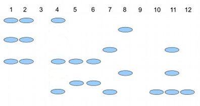
Samples were small red beans (SRB), garbanzo beans (GB), split green pea (SGP), baby lima beans (BLB), and black eye peas (BEP). RAPD primer 1 was applied to samples in lanes 1 – 6; RAPD primer 2 was applied to samples in lane 7 – 12. Lane 1 & 7 = SRB; Lane 2 & 8 = GB; Lanes 3 & 9 = SGP; Lane 4 & 10 = BLB; Lane 5 & 11 = BB; Lane 6 & 12 = BEP.
Here’s how to go from gel documentation to the information needed for genetic distance calculations (see below). I’ll use “1” to indicate presence of a band, “0” to indicate absence of a band, and “?” to indicate no information. For simplicity, I ignored the RF value, but ranked the bands by order of largest (= 1) to smallest (=8) fragment.
We need three pieces of information from the gel to calculate genetic distance.
\(N_{A}\) = the number of markers for taxon A
\(N_{B}\) = the number of markers for taxon B
\(N_{AB}\) = the number of markers in common between A and B (this is the pairwise part — we are comparing taxa two at a time).
First, compare the beans against the same primer. My results for primer 1 are in Table \(\PageIndex{2}\); results for primer 2 are in Table \(\PageIndex{3}\).
| marker | lane 1 | Lane 2 | Lane3 | Lane 4 | Lane 5 | Lane 6 |
| 1 | 1 | 1 | ? | 1 | 0 | 0 |
| 3 | 1 | 1 | ? | 0 | 0 | 0 |
| 5 | 1 | 1 | ? | 1 | 1 | 1 |
| 7 | 0 | 0 | ? | 0 | 1 | 1 |
| marker | Lane 7 | Lane 8 | Lane 9 | Lane 10 | Lane 11 | Lane 12 |
| 2 | 0 | 1 | ? | 0 | 0 | 0 |
| 4 | 1 | 0 | ? | 0 | 1 | 0 |
| 6 | 0 | 1 | ? | 0 | 1 | 0 |
| 8 | 1 | 0 | ? | 1 | 1 | 1 |
From Table \(\PageIndex{2}\) and Table \(\PageIndex{3}\), count \(N_{A} (= N_{B})\) for each taxon. Results are in Table \(\PageIndex{4}\).
| Taxon | No. markers from Primer1 | No. markers from Primer2 | Total |
| SRB | 3 | 2 | 5 |
| GB | 3 | 2 | 5 |
| SGP | ? | ? | ? |
| BLB | 2 | 1 | 3 |
| BB | 2 | 3 | 5 |
| BEP | 2 | 1 | 3 |
As you can see, there is no simple relationship among the taxa; there is no obvious combination of markers that readily group the taxa by similarity. So, I need a computer to help me. I need a measure of genetic distance, a measure that indicates how (dis)similar the different varieties are for our genetic markers. I’ll use a distance calculation that counts only the “present” markers, not the “absent” markers, which is more appropriate for RAPD. I need to get the \(N_{AB}\) values, the number of shared markers between pairs of taxa.
| SRB | GB | BLB | BB | BEP | |
| SRB | 0 | 3 | 3 | 3 | 2 |
| GB | 0 | 2 | 2 | 1 | |
| BLB | 0 | 2 | 2 | ||
| BB | 0 | 3 | |||
| BEP | 0 |
The equation for calculating Nei’s distance is: \[Nei's d = 1 - \left(\frac{N_{AB}}{N_{A} + N_{B} - N_{AB}}\right) \nonumber\]
where \(N_{A}\) = number of bands in taxon “A”, \(N_{B}\) = number of bands in taxon “B”, and \(N_{AB}\) is the number of bands in common between A and B (Nei and Li 1979). Here’s an example calculation.
Let A = SRB and B = GB, then \[Distance = 1 - \left(\frac{3}{5 + 5 - 3}\right) = 0.5714 \nonumber\]
Questions
1. Review all of the different correlation estimates we have introduced in Chapter 16 and construct a table to help you learn. Product moment correlation is presented as example.
| Name of correlation | variable 1 type | variable 2 type | purpose |
| Product moment | ratio | ratio | estimate linear association |