20.12: Phylogenetically independent contrasts
- Page ID
- 45291
\( \newcommand{\vecs}[1]{\overset { \scriptstyle \rightharpoonup} {\mathbf{#1}} } \)
\( \newcommand{\vecd}[1]{\overset{-\!-\!\rightharpoonup}{\vphantom{a}\smash {#1}}} \)
\( \newcommand{\dsum}{\displaystyle\sum\limits} \)
\( \newcommand{\dint}{\displaystyle\int\limits} \)
\( \newcommand{\dlim}{\displaystyle\lim\limits} \)
\( \newcommand{\id}{\mathrm{id}}\) \( \newcommand{\Span}{\mathrm{span}}\)
( \newcommand{\kernel}{\mathrm{null}\,}\) \( \newcommand{\range}{\mathrm{range}\,}\)
\( \newcommand{\RealPart}{\mathrm{Re}}\) \( \newcommand{\ImaginaryPart}{\mathrm{Im}}\)
\( \newcommand{\Argument}{\mathrm{Arg}}\) \( \newcommand{\norm}[1]{\| #1 \|}\)
\( \newcommand{\inner}[2]{\langle #1, #2 \rangle}\)
\( \newcommand{\Span}{\mathrm{span}}\)
\( \newcommand{\id}{\mathrm{id}}\)
\( \newcommand{\Span}{\mathrm{span}}\)
\( \newcommand{\kernel}{\mathrm{null}\,}\)
\( \newcommand{\range}{\mathrm{range}\,}\)
\( \newcommand{\RealPart}{\mathrm{Re}}\)
\( \newcommand{\ImaginaryPart}{\mathrm{Im}}\)
\( \newcommand{\Argument}{\mathrm{Arg}}\)
\( \newcommand{\norm}[1]{\| #1 \|}\)
\( \newcommand{\inner}[2]{\langle #1, #2 \rangle}\)
\( \newcommand{\Span}{\mathrm{span}}\) \( \newcommand{\AA}{\unicode[.8,0]{x212B}}\)
\( \newcommand{\vectorA}[1]{\vec{#1}} % arrow\)
\( \newcommand{\vectorAt}[1]{\vec{\text{#1}}} % arrow\)
\( \newcommand{\vectorB}[1]{\overset { \scriptstyle \rightharpoonup} {\mathbf{#1}} } \)
\( \newcommand{\vectorC}[1]{\textbf{#1}} \)
\( \newcommand{\vectorD}[1]{\overrightarrow{#1}} \)
\( \newcommand{\vectorDt}[1]{\overrightarrow{\text{#1}}} \)
\( \newcommand{\vectE}[1]{\overset{-\!-\!\rightharpoonup}{\vphantom{a}\smash{\mathbf {#1}}}} \)
\( \newcommand{\vecs}[1]{\overset { \scriptstyle \rightharpoonup} {\mathbf{#1}} } \)
\(\newcommand{\longvect}{\overrightarrow}\)
\( \newcommand{\vecd}[1]{\overset{-\!-\!\rightharpoonup}{\vphantom{a}\smash {#1}}} \)
\(\newcommand{\avec}{\mathbf a}\) \(\newcommand{\bvec}{\mathbf b}\) \(\newcommand{\cvec}{\mathbf c}\) \(\newcommand{\dvec}{\mathbf d}\) \(\newcommand{\dtil}{\widetilde{\mathbf d}}\) \(\newcommand{\evec}{\mathbf e}\) \(\newcommand{\fvec}{\mathbf f}\) \(\newcommand{\nvec}{\mathbf n}\) \(\newcommand{\pvec}{\mathbf p}\) \(\newcommand{\qvec}{\mathbf q}\) \(\newcommand{\svec}{\mathbf s}\) \(\newcommand{\tvec}{\mathbf t}\) \(\newcommand{\uvec}{\mathbf u}\) \(\newcommand{\vvec}{\mathbf v}\) \(\newcommand{\wvec}{\mathbf w}\) \(\newcommand{\xvec}{\mathbf x}\) \(\newcommand{\yvec}{\mathbf y}\) \(\newcommand{\zvec}{\mathbf z}\) \(\newcommand{\rvec}{\mathbf r}\) \(\newcommand{\mvec}{\mathbf m}\) \(\newcommand{\zerovec}{\mathbf 0}\) \(\newcommand{\onevec}{\mathbf 1}\) \(\newcommand{\real}{\mathbb R}\) \(\newcommand{\twovec}[2]{\left[\begin{array}{r}#1 \\ #2 \end{array}\right]}\) \(\newcommand{\ctwovec}[2]{\left[\begin{array}{c}#1 \\ #2 \end{array}\right]}\) \(\newcommand{\threevec}[3]{\left[\begin{array}{r}#1 \\ #2 \\ #3 \end{array}\right]}\) \(\newcommand{\cthreevec}[3]{\left[\begin{array}{c}#1 \\ #2 \\ #3 \end{array}\right]}\) \(\newcommand{\fourvec}[4]{\left[\begin{array}{r}#1 \\ #2 \\ #3 \\ #4 \end{array}\right]}\) \(\newcommand{\cfourvec}[4]{\left[\begin{array}{c}#1 \\ #2 \\ #3 \\ #4 \end{array}\right]}\) \(\newcommand{\fivevec}[5]{\left[\begin{array}{r}#1 \\ #2 \\ #3 \\ #4 \\ #5 \\ \end{array}\right]}\) \(\newcommand{\cfivevec}[5]{\left[\begin{array}{c}#1 \\ #2 \\ #3 \\ #4 \\ #5 \\ \end{array}\right]}\) \(\newcommand{\mattwo}[4]{\left[\begin{array}{rr}#1 \amp #2 \\ #3 \amp #4 \\ \end{array}\right]}\) \(\newcommand{\laspan}[1]{\text{Span}\{#1\}}\) \(\newcommand{\bcal}{\cal B}\) \(\newcommand{\ccal}{\cal C}\) \(\newcommand{\scal}{\cal S}\) \(\newcommand{\wcal}{\cal W}\) \(\newcommand{\ecal}{\cal E}\) \(\newcommand{\coords}[2]{\left\{#1\right\}_{#2}}\) \(\newcommand{\gray}[1]{\color{gray}{#1}}\) \(\newcommand{\lgray}[1]{\color{lightgray}{#1}}\) \(\newcommand{\rank}{\operatorname{rank}}\) \(\newcommand{\row}{\text{Row}}\) \(\newcommand{\col}{\text{Col}}\) \(\renewcommand{\row}{\text{Row}}\) \(\newcommand{\nul}{\text{Nul}}\) \(\newcommand{\var}{\text{Var}}\) \(\newcommand{\corr}{\text{corr}}\) \(\newcommand{\len}[1]{\left|#1\right|}\) \(\newcommand{\bbar}{\overline{\bvec}}\) \(\newcommand{\bhat}{\widehat{\bvec}}\) \(\newcommand{\bperp}{\bvec^\perp}\) \(\newcommand{\xhat}{\widehat{\xvec}}\) \(\newcommand{\vhat}{\widehat{\vvec}}\) \(\newcommand{\uhat}{\widehat{\uvec}}\) \(\newcommand{\what}{\widehat{\wvec}}\) \(\newcommand{\Sighat}{\widehat{\Sigma}}\) \(\newcommand{\lt}{<}\) \(\newcommand{\gt}{>}\) \(\newcommand{\amp}{&}\) \(\definecolor{fillinmathshade}{gray}{0.9}\)Introduction
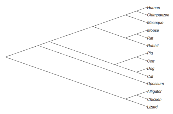
Assumption of independence among the subjects in a study is a key assumption. Comparisons among species are a common experimental approach in evolutionary biology. Typical statistical approaches include use of ANOVA or linear regression approaches. A basic assumption of ANOVA is that sampling units are independent (13.1 – ANOVA assumptions). Prior to the 1980s, it was rarely appreciated in comparative analysis that species are not independent sample units (Harvey and Pagel 1991); evolution produced nested hierarchical relationships among the species. We recognize this with phylogenies (Felsenstein 1985, Harvey and Pagel 1991, Martins 1996, Garland et al 2005). Mice and rats share a more recent common ancestor, and cattle and pigs share a more recent common ancestor, than do mice and cattle, for example. Felsenstein (1985, 1988) is largely credited for making the argument that Type I error is likely if phylogeny is ignored, and, importantly, provided an algorithm: Phylogenetic Independent Contrasts, PIC, which provided a simple way to correct for phylogenetic nonindependence. Felsentein’s landmark 1985 paper has been cited more than ten thousand times (Feb 2024). However, like most innovations, PIC should not be blindly applied in all comparative analysis (e.g., unreplicated evolutionary events, Uyeda et al 2018).
Logic of PIC
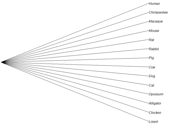
Treating comparative data, e.g., species, as a collection of independent samples implies that the evolutionary history was a spontaneous burst, or star-like phylogeny.

But what nature provides is nonindependence (Fig. \(\PageIndex{2}\), for more about star phylogeny in PIC see discussion in Garland et al 2005), which should be accounted for during statistical analysis.

R package, phytools, ape
Lots of good references on this important subject. For now, see
Chapter 4.2, Estimating rates using independent contrasts, by Dr Luke Harmon
and a tutorial from same author, available at
https://lukejharmon.github.io/ilhabela/instruction/2015/07/02/phylogenetic-independent-contrasts/
Questions
[pending]
References and suggested readings
Felsenstein, J (1985) Phylogenies and the comparative method. American Naturalist 125(1):1-15.
Felsenstein, J. (1988) Phylogenies and quantitative characters. Annual Review of Ecology and Systematics, 19, 445–471.
Garland Jr, T., Bennett, A. F., & Rezende, E. L. (2005). Phylogenetic approaches in comparative physiology. Journal of experimental Biology, 208(16), 3015-3035.
Harvey, P.H. and Pagel, M.D. (1991) The Comparative Method in Evolutionary Biology. Oxford University Press, Oxford, Oxford Series in Ecology and Evolution.
Martins, E.P. (1996) Phylogenies and the Comparative Method in Animal Behavior. Oxford University Press.
Paradis, E. (2012) Analysis of Phylogenetics and Evolution with R (Second Edition). New York: Springer.
Paradis, E. and Schliep, K. (2019) ape 5.0: an environment for modern phylogenetics and evolutionary analyses in R. Bioinformatics, 35, 526–528.
Revell, L. J. (2012) phytools: An R package for phylogenetic comparative biology (and other things). Methods in Ecology and Evolution, 3, 217-223.
Uyeda, J. C., Zenil-Ferguson, R., & Pennell, M. W. (2018). Rethinking phylogenetic comparative methods. Systematic Biology, 67(6), 1091-1109.
Zhang, J., Pei, N., & Mi, X. (2012). phylotools: Phylogenetic tools for Eco-phylogenetics. R package version 0.1, 2.


