16.4: Spearman and other correlations

Introduction

Pearson product moment correlation is used to describe the level of linear association between two variables. There are many types of correlation estimators in addition to the familiar Product Moment Correlation, \(r\).

Spearman rank correlation

If you take the ranks for \(X_{1}\) and the ranks for \(X_{2}\), the correlation of ranks is called Spearman rank correlation, \(r_{s}\). Spearman correlation is a nonparametric statistic. Like the product moment correlation, it can take values between \(-1\) and \(+1\).

For variables \(X_{1}\) and \(X_{2}\), the rank order correlation may be calculated on the ranks as \[\rho = 1 - \frac{6 \sum d_{i}^{2}}{n \left(n^{2}-1\right)} \nonumber\]

where \(d_{i}\) is the difference between the ranks of \(X_{1}\) and \(X_{2}\) for each experimental unit. This formula assumes that there are no tied ranks; if there are, use the equation for the product moment correlation instead (but on the ranks).

R commander has an option to calculate the Spearman rank correlation simply by selecting the check box in the correlation sub menu. However, if the data set is small, it may be easier to just run the correlation in the script window.

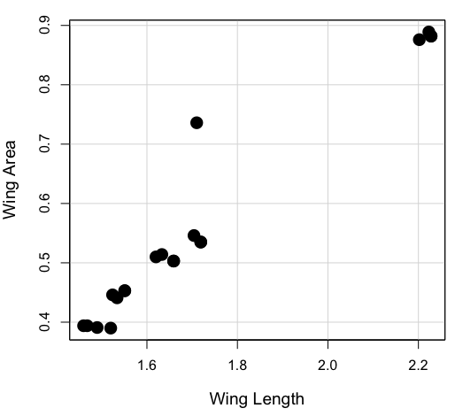
Our example for the product moment correlation was between Drosophila fly wing length and wing area (Table \(\PageIndex{1}\)).

Table \(\PageIndex{1}\). Fly wing lengths and area, units mm and mm², respectively (Dohm pers obs.)

Obs	Student	Length	Area
1	S01	1.524	0.446
2	S01	2.202	0.876
3	S01	1.52	0.39
4	S01	1.62	0.51
5	S01	1.71	0.736
6	S03	1.551	0.453
7	S03	2.228	0.882
8	S03	1.46	0.394
9	S03	1.659	0.503
10	S03	1.719	0.535
11	S05	1.534	0.441
12	S05	2.223	0.889
13	S05	1.49	0.391
14	S05	1.633	0.514
15	S05	1.704	0.546
16	S08	1.551	0.453
17	S08	2.228	0.882
18	S08	1.468	0.394
19	S08	1.659	0.503
20	S08	1.719	0.535

Data were collected by image analysis (ImageJ) of fixed wings to glass slides.

Here’s the scatterplot of the ranks of fly wing length and fly wing area (Fig. \(\PageIndex{1}\)).

Figure \(\PageIndex{1}\): Drosophila wing area (mm²) by wing length (mm).

A nonparametric alternative to the product moment correlation, the Spearman Rank correlation can be obtained directly. The Spearman correlation involves ranking the data, i.e., converting data types, from ratio scale data to ordinal scale, then applying the same formula used for the Product moment correlation to the ranked data. The Spearman correlation would be the choice for testing linear association between two ordinal type variables. It is also appropriate in lieu of the parametric product moment correlation when the statistical assumptions are not met, e.g., normality assumption.

R code

For the Spearman rank correlation, at the R prompt type

cor.test(Area, Length, alternative="two.sided", method="spearman")

R returns with
    Spearman's rank correlation rho

data:  Area and Length
S = 58.699, p-value = 5.139e-11
alternative hypothesis: true rho is not equal to 0
sample estimates:
      rho 
0.9558658

Alternatively, to calculate either correlation, use R Commander.

Rcmdr: Statistics → Summaries→ Correlation test

Example

BM=c(29,29,29,32,32,35,36,38,38,38,40)
Matings=c(0,2,4,4,2,6,3,3,5,8,6)

cor.test(BM,Matings, method="spearman")
Warning in cor.test.default(BM, Matings, method = "spearman") :
  Cannot compute exact p-value with ties

        Spearman's rank correlation rho

data:  BM and Matings
S = 77.7888, p-value = 0.03163
alternative hypothesis: true rho is not equal to 0
sample estimates:
      rho 
0.6464143

cor.test(BM,Matings, method="pearson")

        Pearson's product-moment correlation

data:  BM and Matings
t = 2.6728, df = 9, p-value = 0.02551
alternative hypothesis: true correlation is not equal to 0
95 percent confidence interval:
 0.1087245 0.9042515
sample estimates:
      cor 
0.6652136

Other correlations

Kendall’s tau

Another nonparametric correlation is Kendall’s tau \((\tau)\). Rank the \(X_{1}\) values, then rank the \(X_{2}\) values. Count the number of \(X_{1}, X_{2}\) pairs that have the same rank (concordant pairs) and the number of \(X_{1}, X_{2}\) pairs that do not have the same rank (discordant pairs), Kendall’s tau is then

\[\tau = \frac{(no. \ of \ concordant \ pairs) - (no. \ of \ discordant \ pairs)}{\frac{1}{2} (n-1)} \nonumber\]

where \(n\) is the number of pairs.

Note:

The denominator for \(\tau\) is our familiar number of pairwise comparisons if we take \(k=n\)

We introduced concordant and discordant pairs when we presented McNemar’s test and cross-classified experimental design in Chapter 9.6.

Example: Judging of Science Fair posters

What is the agreement between two judges, A and B, who evaluated the same science fair posters? Posters were evaluated on if the student’s project was hypothesis-based and judges used a Likert-like scale Strongly disagree (1), Somewhat disagree (2), Neutral (3), Somewhat agree (4), Strongly agree (5).

Table \(\PageIndex{2}\). Two judges evaluated six posters for evidence of hypothesis-based project.

Poster	Judge.A	Judge.B
1	5	4
2	2	3
3	4	2
4	3	1
5	2	1
6	4	3

A concordant pair represents a poster ranked higher by both judges, while a disconcordant pair is a poster ranked high by one judge but low by another judge. Poster 1 and poster 5 were concordant pairs.

In R, it is simple to get this correlation directly by invoking the cor.test function and specifying the method equal to kendall. The cor.test assumes that the data are in a matrix, so use the cbind function to bind two vectors together – note the vectors need to have the same number of observations. If the data set is small, it is easier to just enter the data directly in the script window of R commander.

A = c(2,2,3,4,4,5)
B = c(1,3,1,2,3,4)
m = cbind(A,B)
cor.test(A,B, method="kendall")
  Cannot compute exact p-value with ties

        Kendall's rank correlation tau

data:  A and B
z = 1.4113, p-value = 0.1581
alternative hypothesis: true tau is not equal to 0
sample estimates:
      tau 
0.5384615

End of R output

There were no ties in this data set, but we can run the product moment correlation just for comparison:

cor.test(A,B, method="pearson")

        Pearson's product-moment correlation

data:  A and B
t = 1.4649, df = 4, p-value = 0.2168
alternative hypothesis: true correlation is not equal to 0
95 percent confidence interval:
 -0.4239715  0.9478976
sample estimates:
      cor 
0.5909091

End R output

Tetrachoric and Polychoric correlation

Tetrachoric correlations used for binomial outcomes (yes, no), polychoric correlation used for ordinal categorical data like the Likert scale. Introduced by Karl Pearson, commonly applied correlation estimate for Item Analysis in psychometric research. Pyschometrics, a sub-discipline within psychology and now a significant part of education research, is about evaluating assessment tools.

R package psych.

R code: Tetrachoric correlation

tetrachoric(x,y=NULL,correct=.5,smooth=TRUE,global=TRUE,weight=NULL,na.rm=TRUE,
     delete=TRUE)

R code: Polychoric correlation

polychoric(x,smooth=TRUE,global=TRUE,polycor=FALSE,ML=FALSE, std.err=FALSE, 
     weight=NULL,correct=.5,progress=TRUE,na.rm=TRUE,  delete=TRUE)

Polyserial correlation

R package polychor. Used to estimate linear association between a ratio scale variable and an ordinal variable.

R code: Polyserial correlation

polyserial(x,y)

Biserial correlation would be a special case of the polyserial correlation, where ordinal variable is replaced by a dichotomous (binomial) variable.

R code: Polyserial correlation

biserial(x,y)

Intra-class correlation coefficient

Both the ICC and the product moment correlation, \(r\), which we introduced in Chapter 16.1, are measures of strength of linear association between two ratio scale variables (Jinyuan et al 2016). But ICC is more appropriate for association between repeat measures of the same thing, e.g., repeat measures of running speed. In contrast, the product moment correlation can be used to describe association between any two variables, e.g., between repeat measures of running speed, but also between say running speed and maximum jumping height. ICC is used when quantitative measures are organized into paired groups, e.g., before and after on same subjects, or cross-classified designs. ICC was introduced in Chapter 12.3 as part of discussion of repeated measures and random effects. ICC is used extensively to assess reliability of a measurement instrument (Shrout and Fleiss 1979; McGraw and Wong 1996).

Example. Data from Table \(\PageIndex{2}\)

library(psych)
ICC(myJudge, lmer=FALSE)

R output follows

Intraclass correlation coefficients 
                         type  ICC   F df1 df2      p lower bound upper bound
Single_raters_absolute   ICC1 0.40 2.3   5   6  0.166      -0.306        0.84
Single_random_raters     ICC2 0.46 3.9   5   5  0.081      -0.093        0.85
Single_fixed_raters      ICC3 0.59 3.9   5   5  0.081      -0.130        0.90
Average_raters_absolute ICC1k 0.57 2.3   5   6  0.166      -0.880        0.91
Average_random_raters   ICC2k 0.63 3.9   5   5  0.081      -0.205        0.92
Average_fixed_raters    ICC3k 0.74 3.9   5   5  0.081      -0.299        0.95

Number of subjects = 6 Number of Judges = 2
See the help file for a discussion of the other 4 McGraw and Wong estimates

Lots of output, lots of “ICC”. However, rather than explaining each entry, reflect on the type and review the data. Were the posters evaluated repeatedly? Posters were evaluated twice, but only once per judge, so there is a repeated design with respect to the posters. Were judges randomly selected from a population of all possible judges? No evidence was provided to suggest this, so judges were a fixed factor (see Chapter 12.3 and Chapter 14.3). The six ICC estimates reported by R follow discussion in Shrout and Fliess (1979), and our description fits their Case 3: “Each target is rated by each of the same k judges, who are the only judges of interest (p. 421)” Thus, we find ICC for single fixed rater, ICC = 0.59. Note that we would fail to reject the hypothesis that the judges evaluations were associated.

Questions

See Homework 9, Mike’s Workbook for biostatistics