12.3: Fixed effects, random effects, and ICC

Introduction

Within discussions of one-way ANOVA models, the distinction between two general classes of models needs to be made clear by the researcher. The distinction lies in how the levels of the factor are selected. If the researcher selects the levels, then the model is a Fixed Effects Model, also called a Model I ANOVA. On the other hand, if the levels of the factor were selected by random sampling from all possible levels of the factor, then the model is a Random Effects Model, also called a Model II ANOVA.

Here’s an example to help the distinction. Consider an experiment to see if over-the-counter painkillers are as good as prescription pain relievers at reducing numbers of migraines over a six-week period. The researcher selects Tylenol^®, Advil^®, Bayer^® Aspirin, and Sumatriptan (Imitrex^®), the latter an example of a medicine only available by prescription. This is clearly an example of fixed effects; the researcher selected the particular medicines for use.

Random effects, in contrast, implies that the researcher draws up a list of all over-the-counter pain relievers and draws at random three medicines; the researcher would also randomly select from a list of all available prescription medicines.

Fixed effects are probably the more common experimental approaches. To be complete, there is a third class of ANOVA called a Mixed Model or Model III ANOVA, but this type of model only applies to multidimensional ANOVA (e.g., two-way ANOVA or higher), and we reserve our discussion of the Model III until we discuss multidimensional ANOVA (Table \(\PageIndex{1}\)).

Table \(\PageIndex{1}\). ANOVA models.

ANOVA model	Treatments are
I	Fixed effects
II	Random effects
III	Mixed, both fixed & random effects

Although the calculations for the one-way ANOVA under Model I or Model II are the same, the interpretation of the statistical significance is different between the two.

In Model I ANOVA, any statistical difference applies to the differences among the levels selected, but cannot be generalized back to the population. In contrast, statistical significance of the Factor variable in Model II ANOVA cannot be interpreted as specific differences among the levels of the treatment factor, but instead, apply to the population of levels of the factor. In short, Model I ANOVA results apply only to the study, whereas Model II ANOVA results may be interpreted as general effects, applicable to the population.

This distinction between fixed effects and random effects can be confusing, but it has broad implications for how we interpret our results in the short-term. This conceptual distinction between how the levels of the factor are selected also has general implications for our ability to acquire generalizable knowledge by meta-analysis techniques (Hunter and Schmidt 2000). Often we wish to generalize our results: we can do so only if the levels of the factor were randomly selected in the first place from all possible levels of the factor. In reality, this may not often be the case. It is not difficult to find examples in the published literature in which the experimental design is clearly fixed effects (i.e., the researcher selected the treatment levels for a reason), and yet in the discussion of the statistical results, the researcher will lapse into generalizations.

Random Effects Models and Intraclass Correlation Coefficient (ICC)

Model II ANOVA is common in settings in which individuals are measured more than once. For example, in behavioral science or in sports science, subjects are typically measured for the response variable more than once over a course of several trials. Another common setting of Model II ANOVA is where more than one raters are judging an event or even a science project. In all of these cases what we are asking is about whether or not the subjects are consistent, in other words, we are asking about the precision of the instrument or measure.

In the assessment of learning by students, for example, different approaches may be tried and the instructor may wish to investigate whether the interventions can explain changes in test scores. There are an enormous number of articles on reliability measures in the social sciences and you should be aware of a classical paper on reliability by Shrout and Fleiss (1979) (see also McGraw and Wong, 1996). Both the ICC and the product moment correlation, \(r\), which we will introduce in Chapter 16, are measures of strength of linear association between two ratio scale variables (Jinyuan et al 2016). But ICC is more appropriate for association between repeat measures of the same thing, e.g., repeat measures of running speed. In contrast, the product moment correlation can be used to describe association between any two variables, e.g., between repeat measures of running speed, but also between, say, running speed and maximum jumping height. The concept of repeatability of individual behavior or other characteristics is also a common theme in genetics, and so you should not be surprised to learn that the concept actually traces to RA Fisher and his invention of ANOVA and, like in the sociology literature, there are many papers on the use and interpretation of repeatability in the evolutionary biology literature (e.g., Lessels and Boag 1987; Boake 1989; Dohm 2002; Wolak et al 2012).

There are many ways to analyze these kinds of data, but a good way is to treat this problem as a one-way ANOVA with Random Effects. Thus, the Random Effects model permits the partitioning of the variation in the study into two portions: the amount that is due to differences among the subjects or judges or intervention versus the amount that is due to variation within the subjects themselves. The Factor is the Subjects and the levels of the factor are how ever many subjects are measured twice or more for the response variable.

If the subjects performance is repeatable, then the Mean Square Between (Among) Subjects, \(MS_{B}\), component will be greater than the Mean Square Error component, \(MS_{W}\), of the model. There are many measures of repeatability or reliability, but the intraclass correlation coefficient, or ICC, is one of the most common. The ICC may be calculated from the Mean Squares gathered from a Random Effects one-way ANOVA. ICC can take any value between zero and one.

\[ICC = \frac{s_{B}^{2}}{s_{B}^{2} - s_{W}^{2}} \nonumber\]

where \(s_{B}^{2} = MS_{B} - \dfrac{MS_{W}}{k}\) and \(s_{W}^{2} = MS_{W}\)

\(B\) and \(W\) refer, respectively, to the among group (between- or among-groups mean square) and the within group components of variation (error mean square), from the ANOVA. \(MS\) refers to the Mean Squares, and \(k\) is the number of repeat measures for each experimental unit. In this formulation \(k\) is assumed to be the same for each subject.

By example, when a collection of sprinters run a race, if they ran it again, would the outcome be the same, or at least predictable? If the race is run over and over again and the runners cross the finish lines at different times each race, then much of the variation in performance times will be due to race differences largely independent of any performance abilities of the runners themselves and the Mean Square Error term will be large and the Between subjects Mean Square will be small. In contrast, if the race order is preserved race after race: Jenny is first, Ellen is second, Michael is third, and so on, race after race, then differences in performance are largely due to individual differences. In this case, the Between-subjects Mean Square will be large, as will the ICC, whereas the Mean Square for Error will be small.

Can the intraclass correlation be negative?

In theory, no. Values for ICC range between zero and one. The familiar Pearson product moment correlation, Chapter 16, takes any value between \(-1\) and \(+1\). However, in practice, negative values for ICC will result if \(MS_{B} < MS_{W}\).

In other words, if the within-group variability is greater than the among-group variability, then a negative ICC is possible. Small ICC values and few repeats increases the risk of negative ICC estimates. Thus, a negative ICC would be “simply a(n) “unfortunate” estimate (Liljequist et al 2019).

ICC Example

I extracted 15 data points from a figure about nitrogen metabolism in kidney patients following treatment with antibiotics (Figure 1, Mitch et al. 1977). I used a web application called WebPlot Digitizer (https://apps.automeris.io/wpd/), but you can also accomplish this task within R via the digitize package. I was concerned about how steady my hand was using my laptop’s small touch screen, a problem that very much can be answered by thinking statistically, and taking advantage of the ICC. So, rather than taking just one estimate of each point, I repeated the protocol for extracting the points from the figure three times, generating a total of three points for each of the 15 data points (45 points in all). How consistent was I?

Let’s look at the results just for three points, #1, 2, and 3.

In the R script window enter

points = c(1,2,3,1,2,3,1,2,3)

Change points to character so that the ANOVA command will treat the numbers as factor levels.

points = as.character(points)
extracts = c(2.0478, 12.2555, 16.0489, 2.0478, 11.9637, 16.0489, 2.0478, 12.2555, 16.0489)

Make a data frame, assign to an object, e.g., “digitizer”

digitizer = data.frame(points, extracts)

The dataset “digitizer” should now be attached and available to you within Rcmdr. Select digitizer data set and proceed with the one-way ANOVA.

Output from oneway ANOVA command:

Model.1 <- aov(extracts ~ points, data=digitizer)

 summary(Model.1)
            Df    Sum Sq   Mean Sq  F value     Pr(>F)    
points       2 313.38895 156.69448 16562.49 5.9395e-12 ***
Residuals    6   0.05676   0.00946                        
---
Signif. codes:  0 '***' 0.001 '**' 0.01 '*' 0.05 '.' 0.1 ' ' 1

> numSummary(digitizer$extracts , groups=digitizer$points, 
+   statistics=c("mean", "sd"))
         mean           sd data:n
1  2.04780000 0.0000000000      3
2 12.15823333 0.1684708085      3
3 16.04890000 0.0000000000      3

End R output. We need to calculate the ICC. \[ICC = \frac{156.69448 - \frac{0.00946}{3}}{156.69448 - \frac{0.00946}{3} + 0.00946} = 0.9999 \nonumber\]

I’d say that’s pretty repeatable and highly precise measurement!

But is it accurate? You should be able to disentangle accuracy from precision based on our previous discussion (Chapter 3.5), but now in the context of a practical way to quantify precision.

ICC calculations in R

We could continue to calculate the ICC by hand, but better to have a function. Here’s a crack at the function to calculate ICC along with a 95% confidence interval.

myICC <- function(m, k, dfN, dfD) {
 testMe <- anova(m) 
 MSB <- testMe$"Mean Sq"[1]
 MSE <- testMe$"Mean Sq"[2]
 varB <- MSB - MSE/k
 ICC <- varB/(varB+MSE)
 fval <- qf(c(.025), df1=dfN, df2=dfD, lower.tail=TRUE)
 CI = (k*MSE*fval)/(MSB+MSE*(k-1)*fval)
 LCIR = ICC-CI
 UCIR = ICC+CI
 myList = c(ICC, LCIR, UCIR)
 return(myList)
}

The user supplies the ANOVA model object (e.g., Model.1 from our example), \(k\), which is the number of repeats per unit, and degrees of freedom for the among groups comparison (2 in this example), and the error mean square (6 in this case). Our example, run the function

m2ICC = myICC(Model.1, 3, 2,6); m2ICC

and R returns

[1] 0.9999396 0.9999350 0.9999442

with the ICC reported first, 0.9999396, followed by the lower limit (0.9999350) and the upper limit (0.9999442) of the 95% confidence interval.

In lieu of your own function, at several packages available for R will calculate the intraclass correlation coefficient and its variants. These packages are: irr, psy, psych, and rptR. For complex experiments involving multiple predictor variables, these packages are helpful for obtaining the correct ICC calculation (cf Shrout and Fleiss 1979; McGraw and Wong 1996). For the one-way ANOVA it is easier to just extract the information you need from the ANOVA table and run the calculation directly. We do so for a couple of examples.

Example: Are marathon runners consistent more consistent than my commute times?

A marathon is 26 miles, 385 yards long (42.195 kilometers). And yet, tens of thousands of people choose to run in these events. For many, running a marathon is a one-off, the culmination of a personal fitness goal. For others, it’s a passion and a few are simply extraordinary, elite runners who can complete the courses in 2 to 3 hours (Table \(\PageIndex{3}\)). That’s about 12.5 miles per hour. For comparison, my 20-mile commute on the H1 freeway on Oahu typically takes about 40 minutes to complete, or 27 miles per hour (Table \(\PageIndex{2}\), yes, I keep track of my commute times, per Galton’s famous maxim: “Whenever you can, count”).

Table \(\PageIndex{2}\). A sampling of commute speeds, miles per hour (mph), on the H1 freeway during Dr. D’s morning commute

Monday	Tuesday	Wednesday	Thursday	Friday
28.5	23.8	28.5	30.2	26.9
25.8	22.4	29.3	26.2	27.7
26.2	22.6	24.9	24.2	34.3
23.3	26.9	31.3	26.2	30.2

Calculate the ICC for my commute speeds.

Run the one-way ANOVA to get the necessary mean squares and input the values into our ICC function. We have

require(psych)
m2ICC = myICC(AnovaModel.1, 4, 4,11); m2ICC
[1] 0.7390535 0.6061784 0.8719286

Repeatability, as estimated by the ICC, was 0.74 (95% CI 0.606, 0.872), for repeat measures of commute times.

We can ask the same about marathon runners — how consistent from race to race are these runners? The following data are race times drawn from a sample of runners who completed the Honolulu Marathon in both 2016 and 2017 in 2 to 3 hours (times recorded in minutes). In other words, are elite runners consistent?

Table \(\PageIndex{3}\). Honolulu marathon running times (in min.) for eleven repeat, elite runners.

ID	Time 1	Time 2
P1	179.9	192.0
P2	129.9	130.8
P3	128.5	129.6
P4	179.4	179.7
P5	174.3	181.7
P6	177.2	176.2
P7	169.0	173.4
P8	174.1	175.2
P9	175.1	174.2
P10	163.9	175.9
P11	179.3	179.8

After running a one-way ANOVA, here are results for the marathon runners:

m2ICC = myICC(Model.1, 2, 10,11); m2ICC
[1] 0.9780464 0.9660059 0.9900868

Repeatability, as estimated by the ICC, was 0.98 (95% CI 0.966, 0.990), for repeat measures of marathon performance. Put more simply, knowing what a runner did in 2016 I would be able to predict their 2017 race performance with high confidence, 98%!

And now, we compare: the runners are more consistent!

Clearly this is an apples-to-oranges comparison, but it gives us a chance to think about how we might make such comparisons. The ICC will change because of differences among individuals. For example, if individuals are not variable, then xx too little variation.

An example for you to work, from our Measurement Day

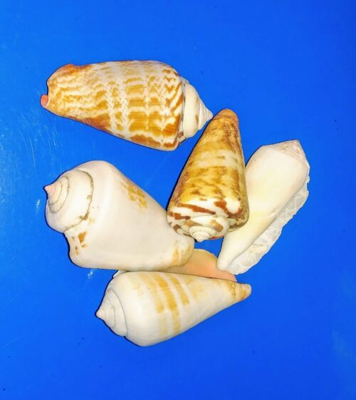
If you recall, we had you calculate length and width measures on shells from samples of gastropod and bivalve species. In the table are repeated measures of shell length, by caliper in mm, for a sample of Conus shells (Fig. \(\PageIndex{1}\) and Table \(\PageIndex{4}\)).

Figure \(\PageIndex{1}\): Conus shells, image by M. Dohm.

Table \(\PageIndex{4}\). Unstacked dataset of repeated length measures on 12 shells.

Sample	Measure 1	Measure 2	Measure 3
1	45.74	46.44	46.79
2	48.79	49.41	53.36
3	52.79	53.45	53.36
4	52.74	53.14	53.14
5	53.25	53.45	53.15
6	53.25	53.64	53.65
7	31.18	31.59	31.44
8	40.73	41.03	41.11
9	43.18	43.23	43.2
10	47.10	47.64	47.64
11	49.53	50.32	50.24
12	53.96	54.50	54.56

---

Questions

1. Consider data in Table \(\PageIndex{2}\), Table \(\PageIndex{3}\), and Table \(\PageIndex{4}\). True or False: The arithmetic mean is an appropriate measure of central tendency. Explain your answer.
2. Enter the shell data into R; it’s best to copy and stack the data in your spreadsheet, then import into R or R Commander. Once imported, don’t forget to change Sample to character, otherwise R will treat Sample as ratio scale data type. Run your one-way ANOVA and calculate the intraclass correlation (ICC) for the dataset. Is the shell length measure repeatable?
3. True or False. A fixed effects ANOVA implies that the researcher selected levels of all treatments.
4. True or False. A random effects ANOVA implies that the researcher selected levels of all treatments.
5. A clinician wishes to compare the effectiveness of three competing brands of blood pressure medication. She takes a random sample of 60 people with high blood pressure and randomly assigns 20 of these 60 people to each of the three brands of blood pressure medication. She then measures the decrease in blood pressure that each person experiences. This is an example of (select all that apply)
   A. a completely randomized experimental design
   B. a randomized block design
   C. a two-factor factorial experiment
   D. a random effects or Type II ANOVA
   E. a mixed model or Type III ANOVA
   F. a fixed effects model or Type I ANOVA
6. A clinician wishes to compare the effectiveness of three competing brands of blood pressure medication. She takes a random sample of 60 people with high blood pressure and randomly assigns 20 of these 60 people to each of the three brands of blood pressure medication. She then measures the blood pressure before treatment and again 6 weeks after treatment for each person. This is an example of (select all that apply)
   A. a completely randomized experimental design
   B. a randomized block design
   C. a two-factor factorial experiment
   D. a random effects or Type II ANOVA
   E. a mixed model or Type III ANOVA
   F. a fixed effects model or Type I ANOVA
7. The advantage of a randomized block design over a completely randomized design is that we may compare treatments by using ________________ experimental units.
   A. randomly selected
   B. the same or nearly the same
   C. independent
   D. dependent
   E. All of the above