
6.10: t-distribution
- Page ID
- 45075

\( \newcommand{\vecs}[1]{\overset { \scriptstyle \rightharpoonup} {\mathbf{#1}} } \)
\( \newcommand{\vecd}[1]{\overset{-\!-\!\rightharpoonup}{\vphantom{a}\smash {#1}}} \)
\( \newcommand{\dsum}{\displaystyle\sum\limits} \)
\( \newcommand{\dint}{\displaystyle\int\limits} \)
\( \newcommand{\dlim}{\displaystyle\lim\limits} \)
\( \newcommand{\id}{\mathrm{id}}\) \( \newcommand{\Span}{\mathrm{span}}\)
( \newcommand{\kernel}{\mathrm{null}\,}\) \( \newcommand{\range}{\mathrm{range}\,}\)
\( \newcommand{\RealPart}{\mathrm{Re}}\) \( \newcommand{\ImaginaryPart}{\mathrm{Im}}\)
\( \newcommand{\Argument}{\mathrm{Arg}}\) \( \newcommand{\norm}[1]{\| #1 \|}\)
\( \newcommand{\inner}[2]{\langle #1, #2 \rangle}\)
\( \newcommand{\Span}{\mathrm{span}}\)
\( \newcommand{\id}{\mathrm{id}}\)
\( \newcommand{\Span}{\mathrm{span}}\)
\( \newcommand{\kernel}{\mathrm{null}\,}\)
\( \newcommand{\range}{\mathrm{range}\,}\)
\( \newcommand{\RealPart}{\mathrm{Re}}\)
\( \newcommand{\ImaginaryPart}{\mathrm{Im}}\)
\( \newcommand{\Argument}{\mathrm{Arg}}\)
\( \newcommand{\norm}[1]{\| #1 \|}\)
\( \newcommand{\inner}[2]{\langle #1, #2 \rangle}\)
\( \newcommand{\Span}{\mathrm{span}}\) \( \newcommand{\AA}{\unicode[.8,0]{x212B}}\)
\( \newcommand{\vectorA}[1]{\vec{#1}} % arrow\)
\( \newcommand{\vectorAt}[1]{\vec{\text{#1}}} % arrow\)
\( \newcommand{\vectorB}[1]{\overset { \scriptstyle \rightharpoonup} {\mathbf{#1}} } \)
\( \newcommand{\vectorC}[1]{\textbf{#1}} \)
\( \newcommand{\vectorD}[1]{\overrightarrow{#1}} \)
\( \newcommand{\vectorDt}[1]{\overrightarrow{\text{#1}}} \)
\( \newcommand{\vectE}[1]{\overset{-\!-\!\rightharpoonup}{\vphantom{a}\smash{\mathbf {#1}}}} \)
\( \newcommand{\vecs}[1]{\overset { \scriptstyle \rightharpoonup} {\mathbf{#1}} } \)
\(\newcommand{\longvect}{\overrightarrow}\)
\( \newcommand{\vecd}[1]{\overset{-\!-\!\rightharpoonup}{\vphantom{a}\smash {#1}}} \)
\(\newcommand{\avec}{\mathbf a}\) \(\newcommand{\bvec}{\mathbf b}\) \(\newcommand{\cvec}{\mathbf c}\) \(\newcommand{\dvec}{\mathbf d}\) \(\newcommand{\dtil}{\widetilde{\mathbf d}}\) \(\newcommand{\evec}{\mathbf e}\) \(\newcommand{\fvec}{\mathbf f}\) \(\newcommand{\nvec}{\mathbf n}\) \(\newcommand{\pvec}{\mathbf p}\) \(\newcommand{\qvec}{\mathbf q}\) \(\newcommand{\svec}{\mathbf s}\) \(\newcommand{\tvec}{\mathbf t}\) \(\newcommand{\uvec}{\mathbf u}\) \(\newcommand{\vvec}{\mathbf v}\) \(\newcommand{\wvec}{\mathbf w}\) \(\newcommand{\xvec}{\mathbf x}\) \(\newcommand{\yvec}{\mathbf y}\) \(\newcommand{\zvec}{\mathbf z}\) \(\newcommand{\rvec}{\mathbf r}\) \(\newcommand{\mvec}{\mathbf m}\) \(\newcommand{\zerovec}{\mathbf 0}\) \(\newcommand{\onevec}{\mathbf 1}\) \(\newcommand{\real}{\mathbb R}\) \(\newcommand{\twovec}[2]{\left[\begin{array}{r}#1 \\ #2 \end{array}\right]}\) \(\newcommand{\ctwovec}[2]{\left[\begin{array}{c}#1 \\ #2 \end{array}\right]}\) \(\newcommand{\threevec}[3]{\left[\begin{array}{r}#1 \\ #2 \\ #3 \end{array}\right]}\) \(\newcommand{\cthreevec}[3]{\left[\begin{array}{c}#1 \\ #2 \\ #3 \end{array}\right]}\) \(\newcommand{\fourvec}[4]{\left[\begin{array}{r}#1 \\ #2 \\ #3 \\ #4 \end{array}\right]}\) \(\newcommand{\cfourvec}[4]{\left[\begin{array}{c}#1 \\ #2 \\ #3 \\ #4 \end{array}\right]}\) \(\newcommand{\fivevec}[5]{\left[\begin{array}{r}#1 \\ #2 \\ #3 \\ #4 \\ #5 \\ \end{array}\right]}\) \(\newcommand{\cfivevec}[5]{\left[\begin{array}{c}#1 \\ #2 \\ #3 \\ #4 \\ #5 \\ \end{array}\right]}\) \(\newcommand{\mattwo}[4]{\left[\begin{array}{rr}#1 \amp #2 \\ #3 \amp #4 \\ \end{array}\right]}\) \(\newcommand{\laspan}[1]{\text{Span}\{#1\}}\) \(\newcommand{\bcal}{\cal B}\) \(\newcommand{\ccal}{\cal C}\) \(\newcommand{\scal}{\cal S}\) \(\newcommand{\wcal}{\cal W}\) \(\newcommand{\ecal}{\cal E}\) \(\newcommand{\coords}[2]{\left\{#1\right\}_{#2}}\) \(\newcommand{\gray}[1]{\color{gray}{#1}}\) \(\newcommand{\lgray}[1]{\color{lightgray}{#1}}\) \(\newcommand{\rank}{\operatorname{rank}}\) \(\newcommand{\row}{\text{Row}}\) \(\newcommand{\col}{\text{Col}}\) \(\renewcommand{\row}{\text{Row}}\) \(\newcommand{\nul}{\text{Nul}}\) \(\newcommand{\var}{\text{Var}}\) \(\newcommand{\corr}{\text{corr}}\) \(\newcommand{\len}[1]{\left|#1\right|}\) \(\newcommand{\bbar}{\overline{\bvec}}\) \(\newcommand{\bhat}{\widehat{\bvec}}\) \(\newcommand{\bperp}{\bvec^\perp}\) \(\newcommand{\xhat}{\widehat{\xvec}}\) \(\newcommand{\vhat}{\widehat{\vvec}}\) \(\newcommand{\uhat}{\widehat{\uvec}}\) \(\newcommand{\what}{\widehat{\wvec}}\) \(\newcommand{\Sighat}{\widehat{\Sigma}}\) \(\newcommand{\lt}{<}\) \(\newcommand{\gt}{>}\) \(\newcommand{\amp}{&}\) \(\definecolor{fillinmathshade}{gray}{0.9}\)Introduction
Student’s \(t\) distribution is a sampling distribution where values are sampled from a normal distributed population, but \(\sigma\), the standard deviation, and \(\mu\), the mean of the population, are not known. When sample size is large and we know the standard deviation, we would use the Z-score to evaluate probabilities of the sample mean. The \(t\)-distribution applies when \(\sigma\) is not known and the sample size is small (e.g., less than 30, per rule of thirty).
According to Wikipedia and sources therein, Student was the pseudonym of William Sealy Gosset, who came up with the t-test and t-distribution.
The equation of the t-test is \[t = \frac{\left(\bar{X} - \mu\right)}{s_{\bar{X}}} \nonumber\]
where the difference between \(\bar{X}\) the sample mean, and \(\mu\), the population mean, is divided by the standard error of the mean, \(s_{\bar{X}}\), defined in Chapter 3.2 and again in Chapter 3.3. This formulation of the \(t\)-test is called the one sample \(t\)-test (Chapter 8.5). We call the result of this calculation the test statistic for \(t\). We evaluate how often that value or greater of a test statistic will occur by applying the \(t\) distribution function.
There are many \(t\)-distributions, actually, one for every degree of freedom. Like the normal distribution, the \(t\) distribution is symmetrical about a mean of zero. But it is stacked up (leptokurtic) around the middle at low degrees of freedom. As degrees of freedom increase, the \(t\) distribution spreads and becomes increasingly like the normal distribution.
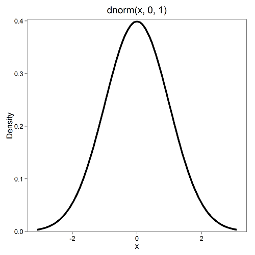
Relationship between \(t\) distribution and standard normal curve
First, here is our standard normal plot, mean = 0, standard deviation = 1
Next, here’s the \(t\)-distribution for five degrees of freedom.

Lets see what happens to the shape of the t-distribution as we increase the degrees of freedom from \(df = 5, 10, 20, 50, 1000, 10000\). The last graphic is the standard normal curve again.
By convention in the Null Hypothesis Significance Testing protocol (NHST), we compare the test statistic to a critical value. The critical value is defined as the value of the test statistic that occurs at the Type I error rate, which is typically set to 5%. We introduced logic of NHST approach in Chapter 6.9 with the chi-square distribution. Again ,this is just an introduction; we teach it now as a sort of mechanical understanding to develop. The justification for this approach to testing of statistical significance is developed in Chapter 8.
| \(df\) | \(\alpha = 0.05\) | \(\alpha = 0.025\) | \(\alpha = 0.01\) |
|---|---|---|---|
| 1 | 6.314 | 12.706 | 31.820 |
| 2 | 2.920 | 4.303 | 6.965 |
| 3 | 2.353 | 3.182 | 4.541 |
| 4 | 2.132 | 2.776 | 3.747 |
| 5 | 2.015 | 2.571 | 3.365 |
Questions
- What happens to the shape of the \(t\) distribution as degrees of freedom are increased from 1 to 5 to 20 to 100?
Be able to answer these questions using the \(t\) table in Appendix 20.4, or using Rcmdr:
- For probability \(\alpha = 5\%\), what is the critical value of the \(t\) distribution (upper tail) for 1 degree of freedom? For \(df = 5\)? For \(df = 20\)? For \(df = 30\)?
- The value of the \(t\) test statistic is given as 12. With 3 degrees of freedom, what is the approximate probability of this value or greater from the \(t\) distribution?