14.2: An Illustrative Data Set

Suppose you’ve become involved in a clinical trial in which you are testing a new antidepressant drug called Joyzepam. In order to construct a fair test of the drug’s effectiveness, the study involves three separate drugs to be administered. One is a placebo, and the other is an existing antidepressant / anti-anxiety drug called Anxifree. A collection of 18 participants with moderate to severe depression are recruited for your initial testing. Because the drugs are sometimes administered in conjunction with psychological therapy, your study includes 9 people undergoing cognitive behavioural therapy (CBT) and 9 who are not. Participants are randomly assigned (doubly blinded, of course) a treatment, such that there are 3 CBT people and 3 no-therapy people assigned to each of the 3 drugs. A psychologist assesses the mood of each person after a 3 month run with each drug: and the overall improvement in each person’s mood is assessed on a scale ranging from −5 to +5.

With that as the study design, let’s now look at what we’ve got in the data file:

load( "./rbook-master/data/clinicaltrial.Rdata" ) # load data
str(clin.trial)

## 'data.frame':    18 obs. of  3 variables:
##  $ drug     : Factor w/ 3 levels "placebo","anxifree",..: 1 1 1 2 2 2 3 3 3 1 ...
##  $ therapy  : Factor w/ 2 levels "no.therapy","CBT": 1 1 1 1 1 1 1 1 1 2 ...
##  $ mood.gain: num  0.5 0.3 0.1 0.6 0.4 0.2 1.4 1.7 1.3 0.6 ...

So we have a single data frame called clin.trial, containing three variables; drug, therapy and mood.gain. Next, let’s print the data frame to get a sense of what the data actually look like.

print( clin.trial )

##        drug    therapy mood.gain
## 1   placebo no.therapy       0.5
## 2   placebo no.therapy       0.3
## 3   placebo no.therapy       0.1
## 4  anxifree no.therapy       0.6
## 5  anxifree no.therapy       0.4
## 6  anxifree no.therapy       0.2
## 7  joyzepam no.therapy       1.4
## 8  joyzepam no.therapy       1.7
## 9  joyzepam no.therapy       1.3
## 10  placebo        CBT       0.6
## 11  placebo        CBT       0.9
## 12  placebo        CBT       0.3
## 13 anxifree        CBT       1.1
## 14 anxifree        CBT       0.8
## 15 anxifree        CBT       1.2
## 16 joyzepam        CBT       1.8
## 17 joyzepam        CBT       1.3
## 18 joyzepam        CBT       1.4

For the purposes of this chapter, what we’re really interested in is the effect of drug on mood.gain. The first thing to do is calculate some descriptive statistics and draw some graphs. In Chapter 5 we discussed a variety of different functions that can be used for this purpose. For instance, we can use the xtabs() function to see how many people we have in each group:

xtabs( ~drug, clin.trial )

## drug
##  placebo anxifree joyzepam 
##        6        6        6

Similarly, we can use the aggregate() function to calculate means and standard deviations for the mood.gain variable broken down by which drug was administered:

aggregate( mood.gain ~ drug, clin.trial, mean )

##       drug mood.gain
## 1  placebo 0.4500000
## 2 anxifree 0.7166667
## 3 joyzepam 1.4833333

aggregate( mood.gain ~ drug, clin.trial, sd )

##       drug mood.gain
## 1  placebo 0.2810694
## 2 anxifree 0.3920034
## 3 joyzepam 0.2136976

Finally, we can use plotmeans() from the gplots package to produce a pretty picture.

library(gplots)
plotmeans(  formula = mood.gain ~ drug,  # plot mood.gain by drug
             data = clin.trial,           # the data frame
             xlab = "Drug Administered",  # x-axis label
             ylab = "Mood Gain",          # y-axis label
             n.label = FALSE              # don't display sample size
 )

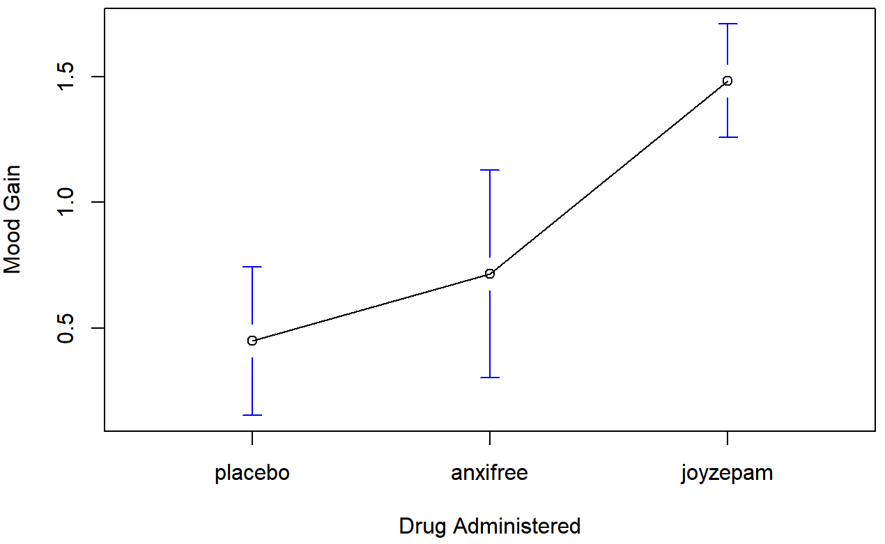
The results are shown in Figure 14.1, which plots the average mood gain for all three conditions; error bars show 95% confidence intervals. As the plot makes clear, there is a larger improvement in mood for participants in the Joyzepam group than for either the Anxifree group or the placebo group. The Anxifree group shows a larger mood gain than the control group, but the difference isn’t as large.

The question that we want to answer is: are these difference “real”, or are they just due to chance?

## Warning: package 'gplots' was built under R version 3.5.2

## 
## Attaching package: 'gplots'

## The following object is masked from 'package:stats':
## 
##     lowess

Figure 14.1: Average mood gain as a function of drug administered. Error bars depict 95% confidence intervals associated with each of the group means.