12.2: Partial Effects

As noted in Chapter 1, multiple regression controls" for the effects of other variables on the dependent variables. This is in order to manage possible spurious relationships, where the variable ZZ influences the value of both XX and YY. Figure \(\PageIndex{1}\) illustrates the nature of spurious relationships between variables.

## Warning in is.na(x): is.na() applied to non-(list or vector) of type
## 'expression'

## Warning in is.na(x): is.na() applied to non-(list or vector) of type
## 'expression'

Figure \(\PageIndex{1}\): Spurious Relationships

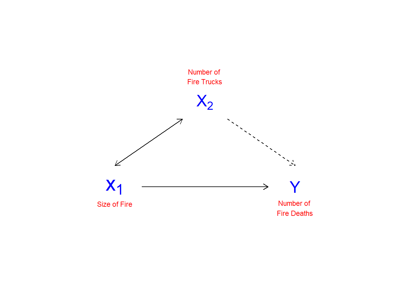
To control for spurious relationships, multiple regression accounts for the partial effects of one XX on another XX. Partial effects deal with the shared variance between YY and the XX’s. This is illustrated in Figure \(\PageIndex{2}\). In this example, the number of deaths resulting from house fires is positively associated with the number of fire trucks that are sent to the scene of the fire. A simple-minded analysis would conclude that if fewer trucks are sent, fewer fire-related deaths would occur. Of course, the number of trucks sent to the fire, and the number of fire-related deaths, are both driven by the magnitude of the fire. An appropriate control for the size of the fire would therefore presumably eliminate the positive association between the number of fire trucks at the scene and the number of deaths (and may even reverse the direction of the relationship, as the larger number of trucks may more quickly suppress the fire).

## Warning: Removed 1 rows containing missing values (geom_point).

## Warning: Removed 1 rows containing missing values (geom_point).

## Warning in is.na(x): is.na() applied to non-(list or vector) of type
## 'expression'

## Warning in is.na(x): is.na() applied to non-(list or vector) of type
## 'expression'

## Warning in is.na(x): is.na() applied to non-(list or vector) of type
## 'expression'

## Warning in is.na(x): is.na() applied to non-(list or vector) of type
## 'expression'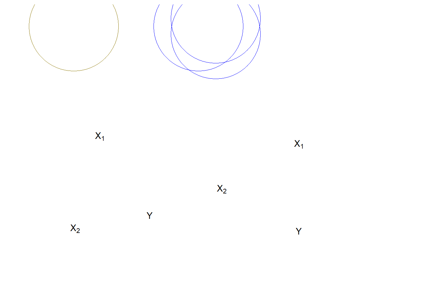

Figure \(\PageIndex{2}\): Partial Effects

In Figure \(\PageIndex{2}\), the Venn diagram on the left shows a pair of XXs that would jointly predict YY better than either XX alone. However, the overlapped area between X1X1 and X2X2 causes some confusion. That would need to be removed to estimate the “pure” effect of X1X1 on YY. The diagram on the right represents a dangerous case. Overall, X1X1+X2X2 explain YY well, but we don`t know how the individual X1X1 or X2X2 influence YY. This clouds our ability to see the effects of either of the XsXs on YY. In the extreme case of wholly overlapping explanations by the IVs, we face the condition of multicolinearity that makes estimation of the partial regression coefficients (the BsBs) impossible.

In calculating the effect of X1X1 on YY, we need to remove the effect of the other XXs on both X1X1 and YY. While multiple regression does this for us, we will walk through an example to illustrate the concepts.

Partial Effects

In a case with two IVs, X1X1 and X2X2

Y=A+B1Xi1+B2Xi2+EiY=A+B1Xi1+B2Xi2+Ei

• Remove the effect of X2X2 and YY

^Yi=A1+B1Xi2+EiY|X2Yi^=A1+B1Xi2+EiY|X2

• Remove the effect of X2X2 on X1X1:

^Xi=A2+B2Xi2+EiX1|X2Xi^=A2+B2Xi2+EiX1|X2

So,

EiY|X2=0+B3EiX1|X2EiY|X2=0+B3EiX1|X2 and B3EiX1|X2=B1Xi1B3EiX1|X2=B1Xi1

As an example, we will use age and ideology to predict perceived climate change risk.

ds.temp <- filter(ds) %>% dplyr::select(glbcc_risk, ideol, age) %>%
  na.omit()

ols1 <- lm(glbcc_risk ~ ideol+age, data = ds.temp)
summary(ols1)

## 
## Call:
## lm(formula = glbcc_risk ~ ideol + age, data = ds.temp)
## 
## Residuals:
##     Min      1Q  Median      3Q     Max 
## -8.7913 -1.6252  0.2785  1.4674  6.6075 
## 
## Coefficients:
##              Estimate Std. Error t value            Pr(>|t|)    
## (Intercept) 11.096064   0.244640  45.357 <0.0000000000000002 ***
## ideol       -1.042748   0.028674 -36.366 <0.0000000000000002 ***
## age         -0.004872   0.003500  -1.392               0.164    
## ---
## Signif. codes:  0 '***' 0.001 '**' 0.01 '*' 0.05 '.' 0.1 ' ' 1
## 
## Residual standard error: 2.479 on 2510 degrees of freedom
## Multiple R-squared:  0.3488, Adjusted R-squared:  0.3483 
## F-statistic: 672.2 on 2 and 2510 DF,  p-value: < 0.00000000000000022

Note that the estimated coefficient for ideology is -1.0427478. To see how multiple regression removes the shared variance we first regress climate change risk on age and create an object ols2.resids of the residuals.

ols2 <- lm(glbcc_risk ~ age, data = ds.temp)
summary(ols2)

## 
## Call:
## lm(formula = glbcc_risk ~ age, data = ds.temp)
## 
## Residuals:
##     Min      1Q  Median      3Q     Max 
## -6.4924 -2.1000  0.0799  2.5376  4.5867 
## 
## Coefficients:
##              Estimate Std. Error t value             Pr(>|t|)    
## (Intercept)  6.933835   0.267116  25.958 < 0.0000000000000002 ***
## age         -0.016350   0.004307  -3.796              0.00015 ***
## ---
## Signif. codes:  0 '***' 0.001 '**' 0.01 '*' 0.05 '.' 0.1 ' ' 1
## 
## Residual standard error: 3.062 on 2511 degrees of freedom
## Multiple R-squared:  0.005706,   Adjusted R-squared:  0.00531 
## F-statistic: 14.41 on 1 and 2511 DF,  p-value: 0.0001504

ols2.resids <- ols2$residuals 

Note that, when modeled alone, the estimated effect of age on glbccrsk is larger (-0.0164) than it was in the multiple regression with ideology (-0.00487). This is because age is correlated with ideology, and – because ideology is also related to glbccrsk – when we don’t “control for” ideology, the age variable carries some of the influence of ideology.

Next, we regress ideology on age and create an object of the residuals.

ols3 <- lm(ideol ~ age, data = ds.temp)
summary(ols3)

## 
## Call:
## lm(formula = ideol ~ age, data = ds.temp)
## 
## Residuals:
##     Min      1Q  Median      3Q     Max 
## -3.9492 -0.8502  0.2709  1.3480  2.7332 
## 
## Coefficients:
##             Estimate Std. Error t value             Pr(>|t|)    
## (Intercept) 3.991597   0.150478  26.526 < 0.0000000000000002 ***
## age         0.011007   0.002426   4.537           0.00000598 ***
## ---
## Signif. codes:  0 '***' 0.001 '**' 0.01 '*' 0.05 '.' 0.1 ' ' 1
## 
## Residual standard error: 1.725 on 2511 degrees of freedom
## Multiple R-squared:  0.00813,    Adjusted R-squared:  0.007735 
## F-statistic: 20.58 on 1 and 2511 DF,  p-value: 0.000005981

ols3.resids <- ols3$residuals

Finally, we regress the residuals from ols2 on the residuals from ols3. Note that this regression does not include an intercept term.

ols4 <- lm(ols2.resids ~ 0 + ols3.resids)
summary(ols4)

## 
## Call:
## lm(formula = ols2.resids ~ 0 + ols3.resids)
## 
## Residuals:
##     Min      1Q  Median      3Q     Max 
## -8.7913 -1.6252  0.2785  1.4674  6.6075 
## 
## Coefficients:
##             Estimate Std. Error t value            Pr(>|t|)    
## ols3.resids -1.04275    0.02866  -36.38 <0.0000000000000002 ***
## ---
## Signif. codes:  0 '***' 0.001 '**' 0.01 '*' 0.05 '.' 0.1 ' ' 1
## 
## Residual standard error: 2.478 on 2512 degrees of freedom
## Multiple R-squared:  0.3451, Adjusted R-squared:  0.3448 
## F-statistic:  1324 on 1 and 2512 DF,  p-value: < 0.00000000000000022

As shown, the estimated BB for EiX1|X2EiX1|X2, matches the estimated BB for ideology in the first regression. What we have done, and what multiple regression does, is clean" both YY and X1X1 (ideology) of their correlations with X2X2 (age) by using the residuals from the bivariate regressions.