7.12: Miscellaneous Topics

To finish this chapter, I have a few topics to discuss that don’t really fit in with any of the other things in this chapter. They’re all kind of useful things to know about, but they are really just “odd topics” that don’t fit with the other examples. Here goes:

problems with floating point arithmetic

If I’ve learned nothing else about transfinite arithmetic (and I haven’t) it’s that infinity is a tedious and inconvenient concept. Not only is it annoying and counterintuitive at times, but it has nasty practical consequences. As we were all taught in high school, there are some numbers that cannot be represented as a decimal number of finite length, nor can they be represented as any kind of fraction between two whole numbers; √2, π and e, for instance. In everyday life we mostly don’t care about this. I’m perfectly happy to approximate π as 3.14, quite frankly. Sure, this does produce some rounding errors from time to time, and if I’d used a more detailed approximation like 3.1415926535 I’d be less likely to run into those issues, but in all honesty I’ve never needed my calculations to be that precise. In other words, although our pencil and paper calculations cannot represent the number π exactly as a decimal number, we humans are smart enough to realise that we don’t care. Computers, unfortunately, are dumb … and you don’t have to dig too deep in order to run into some very weird issues that arise because they can’t represent numbers perfectly. Here is my favourite example:

0.1 + 0.2 == 0.3

## [1] FALSE

Obviously, R has made a mistake here, because this is definitely the wrong answer. Your first thought might be that R is broken, and you might be considering switching to some other language. But you can reproduce the same error in dozens of different programming languages, so the issue isn’t specific to R. Your next thought might be that it’s something in the hardware, but you can get the same mistake on any machine. It’s something deeper than that.

The fundamental issue at hand is floating point arithmetic, which is a fancy way of saying that computers will always round a number to fixed number of significant digits. The exact number of significant digits that the computer stores isn’t important to us:¹³⁰ what matters is that whenever the number that the computer is trying to store is very long, you get rounding errors. That’s actually what’s happening with our example above. There are teeny tiny rounding errors that have appeared in the computer’s storage of the numbers, and these rounding errors have in turn caused the internal storage of 0.1 + 0.2 to be a tiny bit different from the internal storage of 0.3. How big are these differences? Let’s ask R:

0.1 + 0.2 - 0.3

## [1] 5.551115e-17

Very tiny indeed. No sane person would care about differences that small. But R is not a sane person, and the equality operator == is very literal minded. It returns a value of TRUE only when the two values that it is given are absolutely identical to each other. And in this case they are not. However, this only answers half of the question. The other half of the question is, why are we getting these rounding errors when we’re only using nice simple numbers like 0.1, 0.2 and 0.3? This seems a little counterintuitive. The answer is that, like most programming languages, R doesn’t store numbers using their decimal expansion (i.e., base 10: using digits 0, 1, 2 …, 9). We humans like to write our numbers in base 10 because we have 10 fingers. But computers don’t have fingers, they have transistors; and transistors are built to store 2 numbers not 10. So you can see where this is going: the internal storage of a number in R is based on its binary expansion (i.e., base 2: using digits 0 and 1). And unfortunately, here’s what the binary expansion of 0.1 looks like:

.1(decimal)=.00011001100110011...(binary)

and the pattern continues forever. In other words, from the perspective of your computer, which likes to encode numbers in binary,¹³¹ 0.1 is not a simple number at all. To a computer, 0.1 is actually an infinitely long binary number! As a consequence, the computer can make minor errors when doing calculations here.

With any luck you now understand the problem, which ultimately comes down to the twin fact that (1) we usually think in decimal numbers and computers usually compute with binary numbers, and (2) computers are finite machines and can’t store infinitely long numbers. The only questions that remain are when you should care and what you should do about it. Thankfully, you don’t have to care very often: because the rounding errors are small, the only practical situation that I’ve seen this issue arise for is when you want to test whether an arithmetic fact holds exactly numbers are identical (e.g., is someone’s response time equal to exactly 2×0.33 seconds?) This is pretty rare in real world data analysis, but just in case it does occur, it’s better to use a test that allows for a small tolerance. That is, if the difference between the two numbers is below a certain threshold value, we deem them to be equal for all practical purposes. For instance, you could do something like this, which asks whether the difference between the two numbers is less than a tolerance of 10−10

abs( 0.1 + 0.2 - 0.3 ) < 10^-10

## [1] TRUE

To deal with this problem, there is a function called all.equal() that lets you test for equality but allows a small tolerance for rounding errors:

all.equal( 0.1 + 0.2, 0.3 )

## [1] TRUE

recycling rule

There’s one thing that I haven’t mentioned about how vector arithmetic works in R, and that’s the recycling rule. The easiest way to explain it is to give a simple example. Suppose I have two vectors of different length, x and y, and I want to add them together. It’s not obvious what that actually means, so let’s have a look at what R does:

x <- c( 1,1,1,1,1,1 )  # x is length 6
y <- c( 0,1 )          # y is length 2
x + y                  # now add them:

## [1] 1 2 1 2 1 2

As you can see from looking at this output, what R has done is “recycle” the value of the shorter vector (in this case y) several times. That is, the first element of x is added to the first element of y, and the second element of x is added to the second element of y. However, when R reaches the third element of x there isn’t any corresponding element in y, so it returns to the beginning: thus, the third element of x is added to the first element of y. This process continues until R reaches the last element of x. And that’s all there is to it really. The same recycling rule also applies for subtraction, multiplication and division. The only other thing I should note is that, if the length of the longer vector isn’t an exact multiple of the length of the shorter one, R still does it, but also gives you a warning message:

x <- c( 1,1,1,1,1 )    # x is length 5
y <- c( 0,1 )          # y is length 2
x + y                  # now add them:

## Warning in x + y: longer object length is not a multiple of shorter object
## length

## [1] 1 2 1 2 1

introduction to environments

Figure 7.2: The environment panel in Rstudio can actually show you the contents of any loaded package: each package defines a separate environment, so you can select the one you want to look at in this panel.

In this section I want to ask a slightly different question: what is the workspace exactly? This question seems simple, but there’s a fair bit to it. This section can be skipped if you’re not really interested in the technical details. In the description I gave earlier, I talked about the workspace as an abstract location in which R variables are stored. That’s basically true, but it hides a couple of key details. For example, any time you have R open, it has to store lots of things in the computer’s memory, not just your variables. For example, the who() function that I wrote has to be stored in memory somewhere, right? If it weren’t I wouldn’t be able to use it. That’s pretty obvious. But equally obviously it’s not in the workspace either, otherwise you should have seen it! Here’s what’s happening. R needs to keep track of a lot of different things, so what it does is organise them into environments, each of which can contain lots of different variables and functions. Your workspace is one such environment. Every package that you have loaded is another environment. And every time you call a function, R briefly creates a temporary environment in which the function itself can work, which is then deleted after the calculations are complete. So, when I type in search() at the command line

search()

##  [1] ".GlobalEnv"        "package:lsr"       "package:stats"    
##  [4] "package:graphics"  "package:grDevices" "package:utils"    
##  [7] "package:datasets"  "package:methods"   "Autoloads"        
## [10] "package:base"

what I’m actually looking at is a sequence of environments. The first one, ".GlobalEnv" is the technically-correct name for your workspace. No-one really calls it that: it’s either called the workspace or the global environment. And so when you type in objects() or who() what you’re really doing is listing the contents of ".GlobalEnv". But there’s no reason why we can’t look up the contents of these other environments using the objects() function (currently who() doesn’t support this). You just have to be a bit more explicit in your command. If I wanted to find out what is in the package:stats environment (i.e., the environment into which the contents of the stats package have been loaded), here’s what I’d get

head(objects("package:stats"))

## [1] "acf"        "acf2AR"     "add.scope"  "add1"       "addmargins"
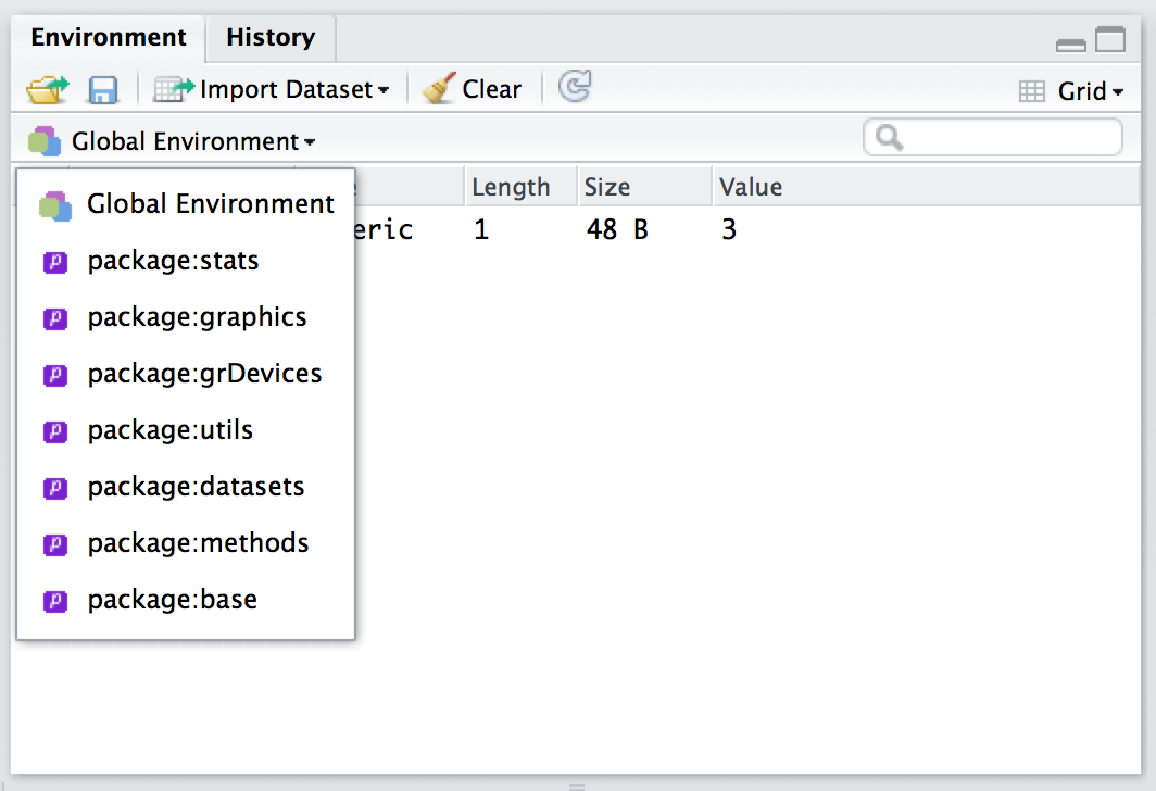
## [6] "aggregate"

where this time I’ve used head() to hide a lot of output because the stats package contains about 500 functions. In fact, you can actually use the environment panel in Rstudio to browse any of your loaded packages (just click on the text that says “Global Environment” and you’ll see a dropdown menu like the one shown in Figure 7.2). The key thing to understand then, is that you can access any of the R variables and functions that are stored in one of these environments, precisely because those are the environments that you have loaded!¹³²

Attaching a data frame

The last thing I want to mention in this section is the attach() function, which you often see referred to in introductory R books. Whenever it is introduced, the author of the book usually mentions that the attach() function can be used to “attach” the data frame to the search path, so you don’t have to use the $ operator. That is, if I use the command attach(df) to attach my data frame, I no longer need to type df$variable, and instead I can just type variable. This is true as far as it goes, but it’s very misleading and novice users often get led astray by this description, because it hides a lot of critical details.

Here is the very abridged description: when you use the attach() function, what R does is create an entirely new environment in the search path, just like when you load a package. Then, what it does is copy all of the variables in your data frame into this new environment. When you do this, however, you end up with two completely different versions of all your variables: one in the original data frame, and one in the new environment. Whenever you make a statement like df$variable you’re working with the variable inside the data frame; but when you just type variable you’re working with the copy in the new environment. And here’s the part that really upsets new users: changes to one version are not reflected in the other version. As a consequence, it’s really easy for R to end up with different value stored in the two different locations, and you end up really confused as a result.

To be fair to the writers of the attach() function, the help documentation does actually state all this quite explicitly, and they even give some examples of how this can cause confusion at the bottom of the help page. And I can actually see how it can be very useful to create copies of your data in a separate location (e.g., it lets you make all kinds of modifications and deletions to the data without having to touch the original data frame). However, I don’t think it’s helpful for new users, since it means you have to be very careful to keep track of which copy you’re talking about. As a consequence of all this, for the purpose of this book I’ve decided not to use the attach() function. It’s something that you can investigate yourself once you’re feeling a little more confident with R, but I won’t do it here.