9.6: 2x2 Between-subjects ANOVA
- Page ID
- 7945
\( \newcommand{\vecs}[1]{\overset { \scriptstyle \rightharpoonup} {\mathbf{#1}} } \)
\( \newcommand{\vecd}[1]{\overset{-\!-\!\rightharpoonup}{\vphantom{a}\smash {#1}}} \)
\( \newcommand{\id}{\mathrm{id}}\) \( \newcommand{\Span}{\mathrm{span}}\)
( \newcommand{\kernel}{\mathrm{null}\,}\) \( \newcommand{\range}{\mathrm{range}\,}\)
\( \newcommand{\RealPart}{\mathrm{Re}}\) \( \newcommand{\ImaginaryPart}{\mathrm{Im}}\)
\( \newcommand{\Argument}{\mathrm{Arg}}\) \( \newcommand{\norm}[1]{\| #1 \|}\)
\( \newcommand{\inner}[2]{\langle #1, #2 \rangle}\)
\( \newcommand{\Span}{\mathrm{span}}\)
\( \newcommand{\id}{\mathrm{id}}\)
\( \newcommand{\Span}{\mathrm{span}}\)
\( \newcommand{\kernel}{\mathrm{null}\,}\)
\( \newcommand{\range}{\mathrm{range}\,}\)
\( \newcommand{\RealPart}{\mathrm{Re}}\)
\( \newcommand{\ImaginaryPart}{\mathrm{Im}}\)
\( \newcommand{\Argument}{\mathrm{Arg}}\)
\( \newcommand{\norm}[1]{\| #1 \|}\)
\( \newcommand{\inner}[2]{\langle #1, #2 \rangle}\)
\( \newcommand{\Span}{\mathrm{span}}\) \( \newcommand{\AA}{\unicode[.8,0]{x212B}}\)
\( \newcommand{\vectorA}[1]{\vec{#1}} % arrow\)
\( \newcommand{\vectorAt}[1]{\vec{\text{#1}}} % arrow\)
\( \newcommand{\vectorB}[1]{\overset { \scriptstyle \rightharpoonup} {\mathbf{#1}} } \)
\( \newcommand{\vectorC}[1]{\textbf{#1}} \)
\( \newcommand{\vectorD}[1]{\overrightarrow{#1}} \)
\( \newcommand{\vectorDt}[1]{\overrightarrow{\text{#1}}} \)
\( \newcommand{\vectE}[1]{\overset{-\!-\!\rightharpoonup}{\vphantom{a}\smash{\mathbf {#1}}}} \)
\( \newcommand{\vecs}[1]{\overset { \scriptstyle \rightharpoonup} {\mathbf{#1}} } \)
\( \newcommand{\vecd}[1]{\overset{-\!-\!\rightharpoonup}{\vphantom{a}\smash {#1}}} \)
\(\newcommand{\avec}{\mathbf a}\) \(\newcommand{\bvec}{\mathbf b}\) \(\newcommand{\cvec}{\mathbf c}\) \(\newcommand{\dvec}{\mathbf d}\) \(\newcommand{\dtil}{\widetilde{\mathbf d}}\) \(\newcommand{\evec}{\mathbf e}\) \(\newcommand{\fvec}{\mathbf f}\) \(\newcommand{\nvec}{\mathbf n}\) \(\newcommand{\pvec}{\mathbf p}\) \(\newcommand{\qvec}{\mathbf q}\) \(\newcommand{\svec}{\mathbf s}\) \(\newcommand{\tvec}{\mathbf t}\) \(\newcommand{\uvec}{\mathbf u}\) \(\newcommand{\vvec}{\mathbf v}\) \(\newcommand{\wvec}{\mathbf w}\) \(\newcommand{\xvec}{\mathbf x}\) \(\newcommand{\yvec}{\mathbf y}\) \(\newcommand{\zvec}{\mathbf z}\) \(\newcommand{\rvec}{\mathbf r}\) \(\newcommand{\mvec}{\mathbf m}\) \(\newcommand{\zerovec}{\mathbf 0}\) \(\newcommand{\onevec}{\mathbf 1}\) \(\newcommand{\real}{\mathbb R}\) \(\newcommand{\twovec}[2]{\left[\begin{array}{r}#1 \\ #2 \end{array}\right]}\) \(\newcommand{\ctwovec}[2]{\left[\begin{array}{c}#1 \\ #2 \end{array}\right]}\) \(\newcommand{\threevec}[3]{\left[\begin{array}{r}#1 \\ #2 \\ #3 \end{array}\right]}\) \(\newcommand{\cthreevec}[3]{\left[\begin{array}{c}#1 \\ #2 \\ #3 \end{array}\right]}\) \(\newcommand{\fourvec}[4]{\left[\begin{array}{r}#1 \\ #2 \\ #3 \\ #4 \end{array}\right]}\) \(\newcommand{\cfourvec}[4]{\left[\begin{array}{c}#1 \\ #2 \\ #3 \\ #4 \end{array}\right]}\) \(\newcommand{\fivevec}[5]{\left[\begin{array}{r}#1 \\ #2 \\ #3 \\ #4 \\ #5 \\ \end{array}\right]}\) \(\newcommand{\cfivevec}[5]{\left[\begin{array}{c}#1 \\ #2 \\ #3 \\ #4 \\ #5 \\ \end{array}\right]}\) \(\newcommand{\mattwo}[4]{\left[\begin{array}{rr}#1 \amp #2 \\ #3 \amp #4 \\ \end{array}\right]}\) \(\newcommand{\laspan}[1]{\text{Span}\{#1\}}\) \(\newcommand{\bcal}{\cal B}\) \(\newcommand{\ccal}{\cal C}\) \(\newcommand{\scal}{\cal S}\) \(\newcommand{\wcal}{\cal W}\) \(\newcommand{\ecal}{\cal E}\) \(\newcommand{\coords}[2]{\left\{#1\right\}_{#2}}\) \(\newcommand{\gray}[1]{\color{gray}{#1}}\) \(\newcommand{\lgray}[1]{\color{lightgray}{#1}}\) \(\newcommand{\rank}{\operatorname{rank}}\) \(\newcommand{\row}{\text{Row}}\) \(\newcommand{\col}{\text{Col}}\) \(\renewcommand{\row}{\text{Row}}\) \(\newcommand{\nul}{\text{Nul}}\) \(\newcommand{\var}{\text{Var}}\) \(\newcommand{\corr}{\text{corr}}\) \(\newcommand{\len}[1]{\left|#1\right|}\) \(\newcommand{\bbar}{\overline{\bvec}}\) \(\newcommand{\bhat}{\widehat{\bvec}}\) \(\newcommand{\bperp}{\bvec^\perp}\) \(\newcommand{\xhat}{\widehat{\xvec}}\) \(\newcommand{\vhat}{\widehat{\vvec}}\) \(\newcommand{\uhat}{\widehat{\uvec}}\) \(\newcommand{\what}{\widehat{\wvec}}\) \(\newcommand{\Sighat}{\widehat{\Sigma}}\) \(\newcommand{\lt}{<}\) \(\newcommand{\gt}{>}\) \(\newcommand{\amp}{&}\) \(\definecolor{fillinmathshade}{gray}{0.9}\)You must be wondering how to calculate a 2x2 ANOVA. We haven’t discussed this yet. We’ve only shown you that you don’t have to do it when the design is a 2x2 repeated measures design (note this is a special case).
We are now going to work through some examples of calculating the ANOVA table for 2x2 designs. We will start with the between-subjects ANOVA for 2x2 designs. We do essentially the same thing that we did before (in the other ANOVAs), and the only new thing is to show how to compute the interaction effect.
Remember the logic of the ANOVA is to partition the variance into different parts. The SS formula for the between-subjects 2x2 ANOVA looks like this:
\[SS_\text{Total} = SS_\text{Effect IV1} + SS_\text{Effect IV2} + SS_\text{Effect IV1xIV2} + SS_\text{Error} \nonumber \]
In the following sections we use tables to show the calculation of each SS. We use the same example as before with the exception that we are turning this into a between-subjects design. There are now 5 different subjects in each condition, for a total of 20 subjects. As a result, we remove the subjects column.
SS Total
We calculate the grand mean (mean of all of the score). Then, we calculate the differences between each score and the grand mean. We square the difference scores, and sum them up. That is \(SS_\text{Total}\), reported in the bottom yellow row.

SS Distraction
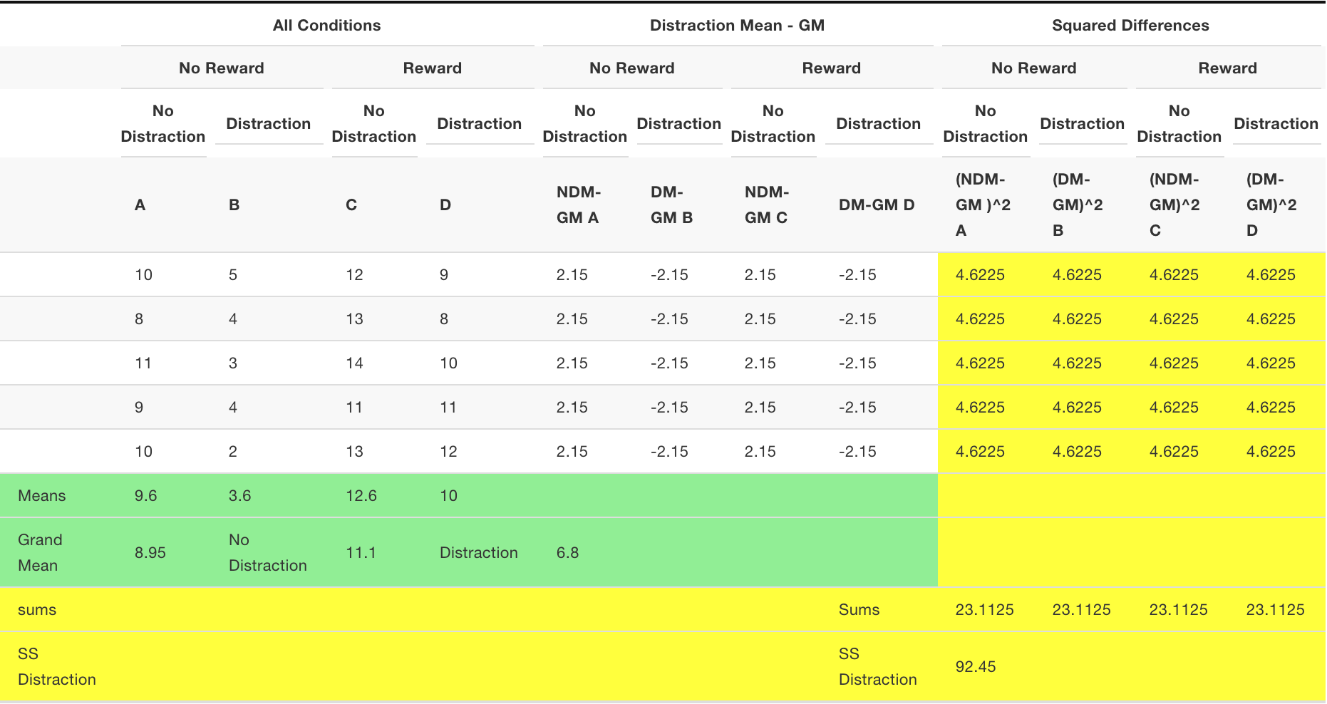
We need to compute the SS for the main effect for distraction. We calculate the grand mean (mean of all of the scores). Then, we calculate the means for the two distraction conditions. Then we treat each score as if it was the mean for it’s respective distraction condition. We find the differences between each distraction condition mean and the grand mean. Then we square the differences and sum them up. That is \(SS_\text{Distraction}\), reported in the bottom yellow row.

These tables are a lot to look at! Notice here, that we first found the grand mean (8.95). Then we found the mean for all the scores in the no-distraction condition (columns A and C), that was 11.1. All of the difference scores for the no-distraction condition are 11.1-8.95 = 2.15. We also found the mean for the scores in the distraction condition (columns B and D), that was 6.8. So, all of the difference scores are 6.8-8.95 = -2.15. Remember, means are the balancing point in the data, this is why the difference scores are +2.15 and -2.15. The grand mean 8.95 is in between the two condition means (11.1 and 6.8), by a difference of 2.15.
SS Reward
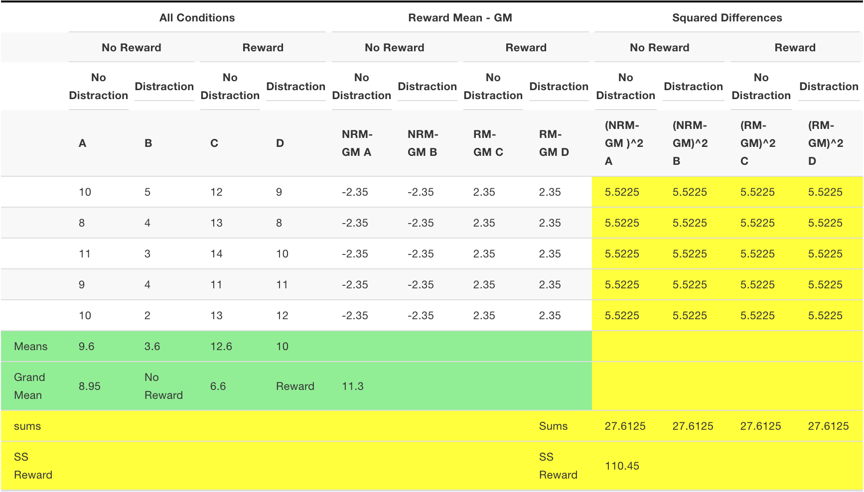
We need to compute the SS for the main effect for reward. We calculate the grand mean (mean of all of the scores). Then, we calculate the means for the two reward conditions. Then we treat each score as if it was the mean for it’s respective reward condition. We find the differences between each reward condition mean and the grand mean. Then we square the differences and sum them up. That is \(SS_\text{Reward}\), reported in the bottom yellow row.

Now we treat each no-reward score as the mean for the no-reward condition (6.6), and subtract it from the grand mean (8.95), to get -2.35. Then, we treat each reward score as the mean for the reward condition (11.3), and subtract it from the grand mean (8.95), to get +2.35. Then we square the differences and sum them up.
SS Distraction by Reward
We need to compute the SS for the interaction effect between distraction and reward. This is the new thing that we do in an ANOVA with more than one IV. How do we calculate the variation explained by the interaction?
The heart of the question is something like this. Do the individual means for each of the four conditions do something a little bit different than the group means for both of the independent variables.
For example, consider the overall mean for all of the scores in the no reward group, we found that to be 6.6 Now, was the mean for each no-reward group in the whole design a 6.6? For example, in the no-distraction group, was the mean for column A (the no-reward condition in that group) also 6.6? The answer is no, it was 9.6. How about the distraction group? Was the mean for the reward condition in the distraction group (column B) 6.6? No, it was 3.6. The mean of 9.6 and 3.6 is 6.6. If there was no hint of an interaction, we would expect that the means for the reward condition in both levels of the distraction group would be the same, they would both be 6.6. However, when there is an interaction, the means for the reward group will depend on the levels of the group from another IV. In this case, it looks like there is an interaction because the means are different from 6.6, they are 9.6 and 3.6 for the no-distraction and distraction conditions. This is extra-variance that is not explained by the mean for the reward condition. We want to capture this extra variance and sum it up. Then we will have measure of the portion of the variance that is due to the interaction between the reward and distraction conditions.
What we will do is this. We will find the four condition means. Then we will see how much additional variation they explain beyond the group means for reward and distraction. To do this we treat each score as the condition mean for that score. Then we subtract the mean for the distraction group, and the mean for the reward group, and then we add the grand mean. This gives us the unique variation that is due to the interaction. We could also say that we are subtracting each condition mean from the grand mean, and then adding back in the distraction mean and the reward mean, that would amount to the same thing, and perhaps make more sense.
Here is a formula to describe the process for each score:
\[\bar{X}_\text{condition} -\bar{X}_\text{IV1} - \bar{X}_\text{IV2} + \bar{X}_\text{Grand Mean} \nonumber \]
Or we could write it this way:
\[\bar{X}_\text{condition} - \bar{X}_\text{Grand Mean} + \bar{X}_\text{IV1} + \bar{X}_\text{IV2} \nonumber \]
When you look at the following table, we apply this formula to the calculation of each of the differences scores. We then square the difference scores, and sum them up to get \(SS_\text{Interaction}\), which is reported in the bottom yellow row.

SS Error
The last thing we need to find is the SS Error. We can solve for that because we found everything else in this formula:
\[SS_\text{Total} = SS_\text{Effect IV1} + SS_\text{Effect IV2} + SS_\text{Effect IV1xIV2} + SS_\text{Error} \nonumber \]
Even though this textbook meant to explain things in a step by step way, we guess you are tired from watching us work out the 2x2 ANOVA by hand. You and me both, making these tables was a lot of work. We have already shown you how to compute the SS for error before, so we will not do the full example here. Instead, we solve for SS Error using the numbers we have already obtained.
\[ \begin{align*} SS_\text{Error} &= SS_\text{Total} - SS_\text{Effect IV1} - SS_\text{Effect IV2} - SS_\text{Effect IV1xIV2} \\[4pt] & = 242.95 - 92.45 - 110.45 - 14.45 \\[4pt] &= 25.6 \end{align*}\]
Check your work
We are going to skip the part where we divide the SSes by their dfs to find the MSEs so that we can compute the three \(F\)-values. Instead, if we have done the calculations of the \(SS\)es correctly, they should be same as what we would get if we used R to calculate the \(SS\)es. Let’s make R do the work, and then compare to check our work.
| Df | Sum Sq | Mean Sq | F value | Pr(>F) | |
|---|---|---|---|---|---|
| Distraction | 1 | 92.45 | 92.45 | 57.78125 | F)" style="vertical-align:middle;">0.0000011 |
| Reward | 1 | 110.45 | 110.45 | 69.03125 | F)" style="vertical-align:middle;">0.0000003 |
| Distraction:Reward | 1 | 14.45 | 14.45 | 9.03125 | F)" style="vertical-align:middle;">0.0083879 |
| Residuals | 16 | 25.60 | 1.60 | NA | F)" style="vertical-align:middle;">NA |
A quick look through the column Sum Sq shows that we did our work by hand correctly. Congratulations to us! Note, this is not the same results as we had before with the repeated measures ANOVA. We conducted a between-subjects design, so we did not get to further partition the SS error into a part due to subject variation and a left-over part. We also gained degrees of freedom in the error term. It turns out with this specific set of data, we find p-values of less than 0.05 for all effects (main effects and the interaction, which was not less than 0.05 using the same data, but treating it as a repeated-measures design)


