3.2: Causality and Invertibility

While a moving average process of order $q$ will always be stationary without conditions on the coefficients $\theta_1$,$\ldots$,$\theta_q$, some deeper thoughts are required in the case of AR($p$) and ARMA($p,q$) processes. For simplicity, we start by investigating the autoregressive process of order one, which is given by the equations $X_t=\phi X_{t-1}+Z_t$ (writing $\phi=\phi_1$). Repeated iterations yield that

$$X_t =\phi X_{t-1}+Z_t =\phi^2X_{t-2}+Z_t+\phi Z_{t-1}=\ldots =\phi^NX_{t-N}+\sum_{j=0}^{N-1}\phi^jZ_{t-j}. \nonumber$$

Letting $N\to\infty$, it could now be shown that, with probability one,

$$X_t=\sum_{j=0}^\infty\phi^jZ_{t-j} \tag{3.2.2}$$

is the weakly stationary solution to the AR(1) equations, provided that $|\phi|<1$. These calculations would indicate moreover, that an autoregressive process of order one can be represented as linear process with coefficients $\psi_j=\phi^j$.

Example $\PageIndex{1}$: Mean and ACVF of an AR(1) process

Since an autoregressive process of order one has been identified as an example of a linear process, one can easily determine its expected value as

$$E[X_t]=\sum_{j=0}^\infty\phi^jE[Z_{t-j}]=0, \qquad t\in\mathbb{Z}. \nonumber$$

For the ACVF, it is obtained that

$$\begin{align*} \gamma(h) &={\rm Cov}(X_{t+h},X_t)\\[.2cm] &=E\left[\sum_{j=0}^\infty\phi^jZ_{t+h-j}\sum_{k=0}^\infty\phi^kZ_{t-k}\right]\\[.2cm] &=\sigma^2\sum_{k=0}^\infty\phi^{k+h}\phi^{k} =\sigma^2\phi^h\sum_{k=0}^\infty\phi^{2k} =\frac{\sigma^2\phi^h}{1-\phi^2}, \end{align*}$$

where $h\geq 0$. This determines the ACVF for all $h$ using that $\gamma(-h)=\gamma(h)$. It is also immediate that the ACF satisfies $\rho(h)=\phi^h$. See also Example 3.1.1 for comparison.

Example $\PageIndex{2}$: Nonstationary AR(1) processes

In Example 1.2.3 we have introduced the random walk as a nonstationary time series. It can also be viewed as a nonstationary AR(1) process with parameter $\phi=1$. In general, autoregressive processes of order one with coefficients $|\phi|>1$ are called {\it explosive}\/ for they do not admit a weakly stationary solution that could be expressed as a linear process. However, one may proceed as follows. Rewrite the defining equations of an AR(1) process as

$$X_t=-\phi^{-1}Z_{t+1}+\phi^{-1}X_{t+1}, \qquad t\in\mathbb{Z}. \nonumber$$

Apply now the same iterations as before to arrive at

$$X_t=\phi^{-N}X_{t+N}-\sum_{j=1}^N\phi^{-j}Z_{t+j},\qquad t\in\mathbb{Z}. \nonumber$$

Note that in the weakly stationary case, the present observation has been described in terms of past innovations. The representation in the last equation however contains only future observations with time lags larger than the present time $t$. From a statistical point of view this does not make much sense, even though by identical arguments as above we may obtain

$$X_t=-\sum_{j=1}^\infty\phi^{-j}Z_{t+j}, \qquad t\in\mathbb{Z}, \nonumber$$

as the weakly stationary solution in the explosive case.

The result of the previous example leads to the notion of causality which means that the process $(X_t: t\in\mathbb{Z})$ has a representation in terms of the white noise $(Z_s: s\leq t)$ and that is hence uncorrelated with the future as given by $(Z_s: s>t)$. We give the definition for the general ARMA case.

Definition: Causality

An ARMA($p,q$) process given by (3.1.1) is causal if there is a sequence $(\psi_j: j\in\mathbb{N}_0)$ such that $\sum_{j=0}^\infty|\psi_j|<\infty$ and

$$X_t=\sum_{j=0}^\infty\psi_jZ_{t-j}, \qquad t\in\mathbb{Z}. \nonumber$$

Causality means that an ARMA time series can be represented as a linear process. It was seen earlier in this section how an AR(1) process whose coefficient satisfies the condition $|\phi|<1$ can be converted into a linear process. It was also shown that this is impossible if $|\phi|>1$. The conditions on the autoregressive parameter $\phi$ can be restated in terms of the corresponding autoregressive polynomial $\phi(z)=1-\phi z$ as follows. It holds that

$|\phi|<1$ if and only if $\phi(z)\not=0$ for all $|z|\leq 1, \\[.2cm]$

$|\phi|>1$ if and only if $\phi(z)\not=0$ for all $|z|\geq 1$.

It turns out that the characterization in terms of the zeroes of the autoregressive polynomials carries over from the AR(1) case to the general ARMA($p,q$) case. Moreover, the $\psi$-weights of the resulting linear process have an easy representation in terms of the polynomials $\phi(z)$ and $\theta(z)$. The result is summarized in the next theorem.

Theorem 3.2.1

Let $(X_t: t\in\mathbb{Z})$ be an ARMA($p,q$) process such that the polynomials $\phi(z)$ and $\theta(z)$ have no common zeroes. Then $(X_t\colon t\in\mathbb{Z})$ is causal if and only if $\phi(z)\not=0$ for all $z\in\mathbb{C}$ with $|z|\leq 1$. The coefficients $(\psi_j: j\in\mathbb{N}_0)$ are determined by the power series expansion

$$\psi(z)=\sum_{j=0}^\infty\psi_jz^j=\frac{\theta(z)}{\phi(z)}, \qquad |z|\leq 1. \nonumber$$

A concept closely related to causality is invertibility. This notion is motivated with the following example that studies properties of a moving average time series of order 1.

Example $\PageIndex{3}$

Let $(X_t\colon t\in\mathbb{N})$ be an MA(1) process with parameter $\theta=\theta_1$. It is an easy exercise to compute the ACVF and the ACF as

$$\gamma(h)=\left\{ \begin{array}{l@{\quad}l} (1+\theta^2)\sigma^2, & h=0, \\ \theta\sigma^2, & h=1 \\ 0 & h>1, \end{array}\right. \qquad \rho(h)=\left\{ \begin{array}{l@{\quad}l} 1 & h=0.\\ \displaystyle\theta(1+\theta^2)^{-1}, & h=1. \\ 0 & h>1. \end{array}\right. \nonumber$$

These results lead to the conclusion that $\rho(h)$ does not change if the parameter $\theta$ is replaced with $\theta^{-1}$. Moreover, there exist pairs $(\theta,\sigma^2)$ that lead to the same ACVF, for example $(5,1)$ and $(1/5,25)$. Consequently, we arrive at the fact that the two MA(1) models

$$X_t=Z_t+\frac 15Z_{t-1},\qquad t\in\mathbb{Z}, \qquad (Z_t\colon t\in\mathbb{Z})\sim\mbox{iid }{\cal N}(0,25), \nonumber$$

and

$$X_t=\tilde{Z}_t+5\tilde{Z}_{t-1},\qquad t\in\mathbb{Z}, \qquad (\tilde{Z}\colon t\in\mathbb{Z})\sim\mbox{iid }{\cal N}(0,1), \nonumber$$

are indistinguishable because we only observe $X_t$ but not the noise variables $Z_t$ and $\tilde{Z}_t$.

For convenience, the statistician will pick the model which satisfies the invertibility criterion which is to be defined next. It specifies that the noise sequence can be represented as a linear process in the observations.

Definition: Invertibility

An ARMA($p,q$) process given by (3.1.1) is invertible if there is a sequence $(\pi_j\colon j\in\mathbb{N}_0)$ such that $\sum_{j=0}^\infty|\pi_j|<\infty$ and

$$Z_t=\sum_{j=0}^\infty\pi_jX_{t-j},\qquad t\in\mathbb{Z}. \nonumber$$

Theorem 3.2.2

Let $(X_t: t\in\mathbb{Z})$ be an ARMA($p,q$) process such that the polynomials $\phi(z)$ and $\theta(z)$ have no common zeroes. Then $(X_t\colon t\in\mathbb{Z})$ is invertible if and only if $\theta(z)\not=0$ for all $z \in\mathbb{C}$ with $|z|\leq 1$. The coefficients $(\pi_j)_{j\in\mathbb{N}_0}$ are determined by the power series expansion

$$\pi(z)=\sum_{j=0}^\infty\pi_jz^j=\frac{\phi(z)}{\theta(z)}, \qquad |z|\leq 1. \nonumber$$

From now on it is assumed that all ARMA sequences specified in the sequel are causal and invertible unless explicitly stated otherwise. The final example of this section highlights the usefulness of the established theory. It deals with parameter redundancy and the calculation of the causality and invertibility sequences $(\psi_j\colon j\in\mathbb{N}_0)$ and $(\pi_j\colon j\in\mathbb{N}_0)$.

Example $\PageIndex{4}$: Parameter redundancy

Consider the ARMA equations

$$X_t=.4X_{t-1}+.21X_{t-2}+Z_t+.6Z_{t-1}+.09Z_{t-2}, \nonumber$$

which seem to generate an ARMA(2,2) sequence. However, the autoregressive and moving average polynomials have a common zero:

$$\begin{align*} \tilde{\phi}(z)&=1-.4z-.21z^2=(1-.7z)(1+.3z), \\[.2cm] \tilde{\theta}(z)&=1+.6z+.09z^2=(1+.3z)^2. \end{align*}$$

Therefore, one can reset the ARMA equations to a sequence of order (1,1) and obtain

$$X_t=.7X_{t-1}+Z_t+.3Z_{t-1}. \nonumber$$

Now, the corresponding polynomials have no common roots. Note that the roots of $\phi(z)=1-.7z$ and $\theta(z)=1+.3z$ are $10/7>1$ and $-10/3<-1$, respectively. Thus Theorems 3.2.1 and 3.2.2 imply that causal and invertible solutions exist. In the following, the corresponding coefficients in the expansions

$$X_t=\sum_{j=0}^\infty\psi_jZ_{t-j} \qquad and \qquad Z_t=\sum_{j=0}^\infty\pi_jX_{t-j}, \qquad t\in\mathbb{Z}, \nonumber$$

are calculated. Starting with the causality sequence $(\psi_j: j\in\mathbb{N}_0)$. Writing, for $|z|\leq 1$,

$$\sum_{j=0}^\infty\psi_jz^j =\psi(z) =\frac{\theta(z)}{\phi(z)} =\frac{1+.3z}{1-.7z} =(1+.3z)\sum_{j=0}^\infty(.7z)^j, \nonumber$$

it can be obtained from a comparison of coefficients that

$$\psi_0=1 \qquad and \qquad \psi_j=(.7+.3)(.7)^{j-1}=(.7)^{j-1}, \qquad j\in\mathbb{N}. \nonumber$$

Similarly one computes the invertibility coefficients $(\pi_j: j\in\mathbb{N}_0)$ from the equation

$$\sum_{j=0}^\infty\pi_jz^j =\pi(z) =\frac{\phi(z)}{\theta(z)} =\frac{1-.7z}{1+.3z} =(1-.7z)\sum_{j=0}^\infty(-.3z)^j \nonumber$$

($|z|\leq 1$) as

$$\pi_0=1 \qquad and \qquad \pi_j=(-1)^j(.3+.7)(.3)^{j-1}=(-1)^j(.3)^{j-1}. \nonumber$$

Together, the previous calculations yield to the explicit representations

$$X_t=Z_t+\sum_{j=1}^\infty(.7)^{j-1}Z_{t-j} \qquad and \qquad Z_t=X_t+\sum_{j=1}^\infty(-1)^j(.3)^{j-1}X_{t-j}. \nonumber$$

In the remainder of this section, a general way is provided to determine the weights $(\psi_j\colon j\geq 1)$ for a causal ARMA($p,q$) process given by $\phi(B)X_t=\theta(B)Z_t$, where $\phi(z)\not=0$ for all $z\in\mathbb{C}$ such that $|z|\leq 1$. Since $\psi(z)=\theta(z)/\phi(z)$ for these $z$, the weight $\psi_j$ can be computed by matching the corresponding coefficients in the equation $\psi(z)\phi(z)=\theta(z)$, that is,

$$(\psi_0+\psi_1z+\psi_2z^2+\ldots)(1-\phi_1z-\ldots-\phi_pz^p) = 1+\theta_1z+\ldots+\theta_qz^q. \nonumber$$

Recursively solving for $\psi_0,\psi_1,\psi_2,\ldots$ gives

$$\begin{align*} \psi_0&=1, \\ \psi_1-\phi_1\psi_0&=\theta_1, \\ \psi_2-\phi_1\psi_1-\phi_2\psi_0&=\theta_2, \end{align*}$$

and so on as long as $j<\max\{p,q+1\}$. The general solution can be stated as

$$\psi_j-\sum_{k=1}^j\phi_k\psi_{j-k}=\theta_j, \qquad 0\leq j<\max\{p,q+1\}, \tag{3.2.1}\\[.2cm]$$

$$\psi_j-\sum_{k=1}^p\phi_k\psi_{j-k}=0, \qquad \phantom{0\leq} j\geq\max\{p,q+1\},\tag{3.2.2}$$

if we define $\phi_j=0$ if $j>p$ and $\theta_j=0$ if $j>q$. To obtain the coefficients $\psi_j$ one therefore has to solve the homogeneous linear difference equation (3.2.2) subject to the initial conditions specified by (3.2.1). For more on this subject, see Section 3.6 of Brockwell and Davis (1991) and Section 3.3 of Shumway and Stoffer (2006).

R calculations

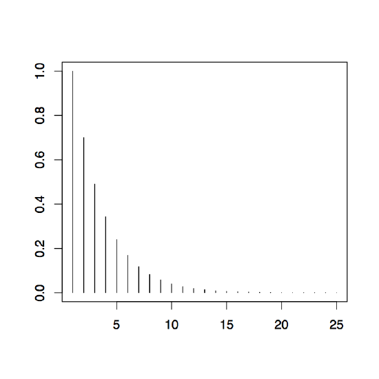
In R, these computations can be performed using the command ARMAtoMA. For example, one can use the commands

>ARMAtoMA(ar=.7,ma=.3,25)

>plot(ARMAtoMA(ar=.7,ma=.3,25))

which will produce the output displayed in Figure 3.4. The plot shows nicely the exponential decay of the $\psi$-weights which is typical for ARMA processes. The table shows row-wise the weights $\psi_0,\ldots,\psi_{24}$. This is enabled by the choice of 25 in the argument of the function ARMAtoMA.

1.0000000000	0.7000000000	0.4900000000	0.3430000000	0.2401000000
0.1680700000	0.1176490000	0.0823543000	0.0576480100	0.0403536070
0.0282475249	0.0197732674	0.0138412872	0.0096889010	0.0067822307
0.0047475615	0.0033232931	0.0023263051	0.0016284136	0.0011398895
0.0007979227	0.0005585459	0.0003909821	0.0002736875	0.0001915812

Figure 3.4: The R output for the ARMA(1,1) process of Example 3.2.4

Contributers

• Alexander Aue (Department of Statistics, University of California, Davis)