6.7: Least Squares Estimation

The previous results used the lm function as a “black box” to generate the estimated coefficients. The lines produced probably look reasonable but you could imagine drawing other lines that might look equally plausible. Because we are interested in explaining variation in the response variable, we want a model that in some sense minimizes the residuals \((e_i = y_i-\widehat{y}_i)\) and explains the responses as well as possible, in other words has \(y_i-\widehat{y}_i\) as small as possible. We can’t just add these \(e_i\)’s up because it would always be 0 (remember why we use the variance to measure spread from introductory statistics?). We use a similar technique in regression, we find the regression line that minimizes the squared residuals \(e^2_i = (y_i-\widehat{y}_i)^2\) over all the observations, minimizing the Sum of Squared Residuals\(\boldsymbol{ = \Sigma e^2_i}\). Finding the estimated regression coefficients that minimize the sum of squared residuals is called least squares estimation and provides us a reasonable method for finding the “best” estimated regression line of all the possible choices.

For the Beers vs BAC data, Figure 6.16 shows the result of a search for the optimal slope coefficient between values of 0 and 0.03. The plot shows how the sum of the squared residuals was minimized for the value that lm returned at 0.018. The main point of this is that if any other slope coefficient was tried, it did not do as good on the least squares criterion as the least squares estimates.

Figure 6.16: Plot of sum of squared residuals vs possible slope coefficients for Beers vs BAC data, with vertical line for the least squares estimate that minimizes the sum of squared residuals.

Sometimes it is helpful to have a go at finding the estimates yourself. If you install and load the tigerstats (Robinson and White 2020) and manipulate (Allaire 2014) packages in RStudio and then run FindRegLine(), you get a chance to try to find the optimal slope and intercept for a fake data set. Click on the “sprocket” icon in the upper left of the plot and you will see something like Figure 6.17. This interaction can help you see how the residuals are being measuring in the \(y\)-direction and appreciate that lm takes care of this for us.

> library(tigerstats)
> library(manipulate)
> FindRegLine()

Equation of the regression line is:
y = 4.34 + -0.02x

Your final score is 13143.99
Thanks for playing!

Figure 6.17: Results of running FindRegLine() where I didn’t quite find the least squares line. The correct line is the bold (red) line and produced a smaller sum of squared residuals than the guessed thinner (black) line.

It ends up that the least squares criterion does not require a search across coefficients or trial and error – there are some “simple” equations available for calculating the estimates of the \(y\)-intercept and slope:

\[b_1 = \frac{\Sigma_i(x_i-\bar{x})(y_i-\bar{y})}{\Sigma_i(x_i-\bar{x})^2} = r\frac{s_y}{s_x} \text{ and } b_0 = \bar{y} - b_1\bar{x}.\]

You will never need to use these equations but they do inform some properties of the regression line. The slope coefficient, \(b_1\), is based on the variability in \(x\) and \(y\) and the correlation between them. If \(\boldsymbol{r} = 0\), then the slope coefficient will also be 0. The intercept is a function of the means of \(x\) and \(y\) and what the estimated slope coefficient is. If the slope coefficient, \(\boldsymbol{b_1}\), is 0, then \(\boldsymbol{b_0 = \bar{y}}\) (which is just the mean of the response variable for all observed values of \(x\) – this is a very boring model!). The slope is 0 when the correlation is 0. So when there is no linear relationship between \(x\) and \(y\) (\(r = 0\)), the least squares regression line is a horizontal line with height \(\bar{y}\), and the line produces the same fitted values for all \(x\) values. You can also think about this as when there is no relationship between \(x\) and \(y\), the best prediction of \(y\) is the mean of the \(y\)-values and it doesn’t change based on the values of \(x\). It is less obvious in these equations, but they also imply that the regression line ALWAYS goes through the point \(\boldsymbol{(\bar{x},\bar{y}).}\) It provides a sort of anchor point for all regression lines.

For one more example, we can revisit the Montana wildfire areas burned (log-hectares) and the average summer temperature (degrees F), which had \(\boldsymbol{r} = 0.81\). The interpretations of the different parts of the regression model follow the least squares estimation provided by lm:

fire1 <- lm(loghectares ~ Temperature, data = mtfires)
summary(fire1)

## 
## Call:
## lm(formula = loghectares ~ Temperature, data = mtfires)
## 
## Residuals:
##     Min      1Q  Median      3Q     Max 
## -3.0822 -0.9549  0.1210  1.0007  2.4728 
## 
## Coefficients:
##             Estimate Std. Error t value Pr(>|t|)
## (Intercept) -69.7845    12.3132  -5.667 1.26e-05
## Temperature   1.3884     0.2165   6.412 2.35e-06
## 
## Residual standard error: 1.476 on 21 degrees of freedom
## Multiple R-squared:  0.6619, Adjusted R-squared:  0.6458 
## F-statistic: 41.12 on 1 and 21 DF,  p-value: 2.347e-06

• Regression Equation (Completely Specified):
  • Estimated model: \(\widehat{\text{log(Ha)}} = -69.78 + 1.39\cdot\text{Temp}\)
  • Or \(\widehat{y} = -69.78 + 1.39x\) with Y = log(Ha) and X = Temperature
• Response Variable: Yearly log Hectares burned by wildfires
• Explanatory Variable: Average Summer Temperature
• Estimated \(y\)-Intercept (\(b_0\)): -69.78
• Estimated slope (\(b_1\)): 1.39
• Slope Interpretation: For a 1 degree Fahrenheit increase in Average Summer Temperature we would expect, on average, a 1.39 log(Hectares) \(\underline{change}\) in log(Hectares) burned in Montana.
• \(Y\)-intercept Interpretation: If temperature were 0 degrees F, we would expect -69.78 log(Hectares) burned on average in Montana.

One other use of regression equations is for prediction. It is a trivial exercise (or maybe not – we’ll see when you try it!) to plug an \(x\)-value of interest into the regression equation and get an estimate for \(y\) at that \(x\). Basically, the regression lines displayed in the scatterplots show the predictions from the regression line across the range of \(x\text{'s}\). Formally, prediction involves estimating the response for a particular value of \(x\). We know that it won’t be perfect but it is our best guess. Suppose that we are interested in predicting the log-area burned for a summer that had an average temperature of \(59^\circ\text{F}\). If we plug \(59^\circ\text{F}\) into the regression equation, \(\widehat{\text{log(Ha)}} = -69.78 + 1.39\bullet \text{Temp}\), we get

\[\begin{array}{rl} \\ \require{cancel} \widehat{\log(\text{Ha})}& = -69.78\text{ log-hectares }+ 1.39\text{ log-hectares}/^\circ \text{F}\bullet 59^\circ\text{F} \\& = -69.78\text{ log-hectares } +1.39\text{ log-hectares}/\cancel{^\circ \text{F}}\bullet 59\cancel{^\circ \text{F}} \\& = 12.23 \text{ log-hectares} \\ \end{array}\]

We did not observe any summers at exactly \(x = 59\) but did observe some nearby and this result seems relatively reasonable.

Now suppose someone asks you to use this equation for predicting \(\text{Temperature} = 65^\circ F\). We can run that through the equation: \(-69.78 + 1.39*65 = 20.57\) log-hectares. But can we trust this prediction? We did not observe any summers over 60 degrees F so we are now predicting outside the scope of our observations – performing extrapolation. Having a scatterplot in hand helps us to assess the range of values where we can reasonably use the equation – here between 54 and 60 degrees F seems reasonable.

mtfires %>% ggplot(mapping = aes(x = Temperature, y = loghectares)) +
  geom_point(aes(color = Year), size = 2.5) +
  geom_smooth(method = "lm") +
  theme_bw() +
  scale_color_viridis() +
  labs(title = "Scatterplot with regression line for Area burned vs 
       Temperature, colored by year")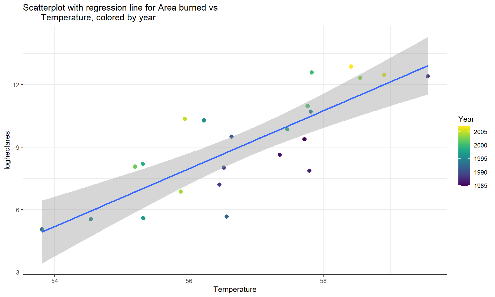

Figure 6.18: Scatterplot of log-hectares burned versus temperature with estimated regression line. Information on the year of each observation is added using a local aesthetic inside geom_point to color the points on a color gradient based on Year.