4.6: Pushing Two-Way ANOVA to the limit - Un-replicated designs and Estimability

In some situations, it is too expensive or impossible to replicate combinations of treatments and only one observation at each combination of the two explanatory variables, A and B, is possible. In these situations, even though we have information about all combinations of A and B, it is no longer possible to test for an interaction. Our regular rules for degrees of freedom show that we have nothing left for the error degrees of freedom and so we have to drop the interaction and call that potential interaction variability “error”.

Without replication we can still perform an analysis of the responses and estimate all the coefficients in the interaction model but an issue occurs with trying to calculate the interaction \(F\)-test statistic – we run out of degrees of freedom for the error. To illustrate these methods, the paper towel example is revisited except that only one response for each combination is used. Now the entire data set can be easily printed out:

ptR <- read_csv("http://www.math.montana.edu/courses/s217/documents/ptR.csv")
ptR <- ptR %>% mutate(dropsf = factor(drops),
                      brand = factor(brand))
ptR

## # A tibble: 6 × 4
##   brand drops responses dropsf
##   <fct> <dbl>     <dbl> <fct> 
## 1 B1       10     1.91  10    
## 2 B2       10     3.05  10    
## 3 B1       20     0.774 20    
## 4 B2       20     2.84  20    
## 5 B1       30     1.56  30    
## 6 B2       30     0.547 30

Upon first inspection the interaction plot in Figure 4.21 looks like there might be some interesting interactions present with lines that look to be non-parallel. But remember now that there is only a single observation at each combination of the brands and water levels so there is not much power to detect differences in this sort of situation and no replicates at any combinations of levels that allow estimation of SEs so no bands are produced in the plot.

Figure 4.21: Interaction plot in paper towel data set with no replication.

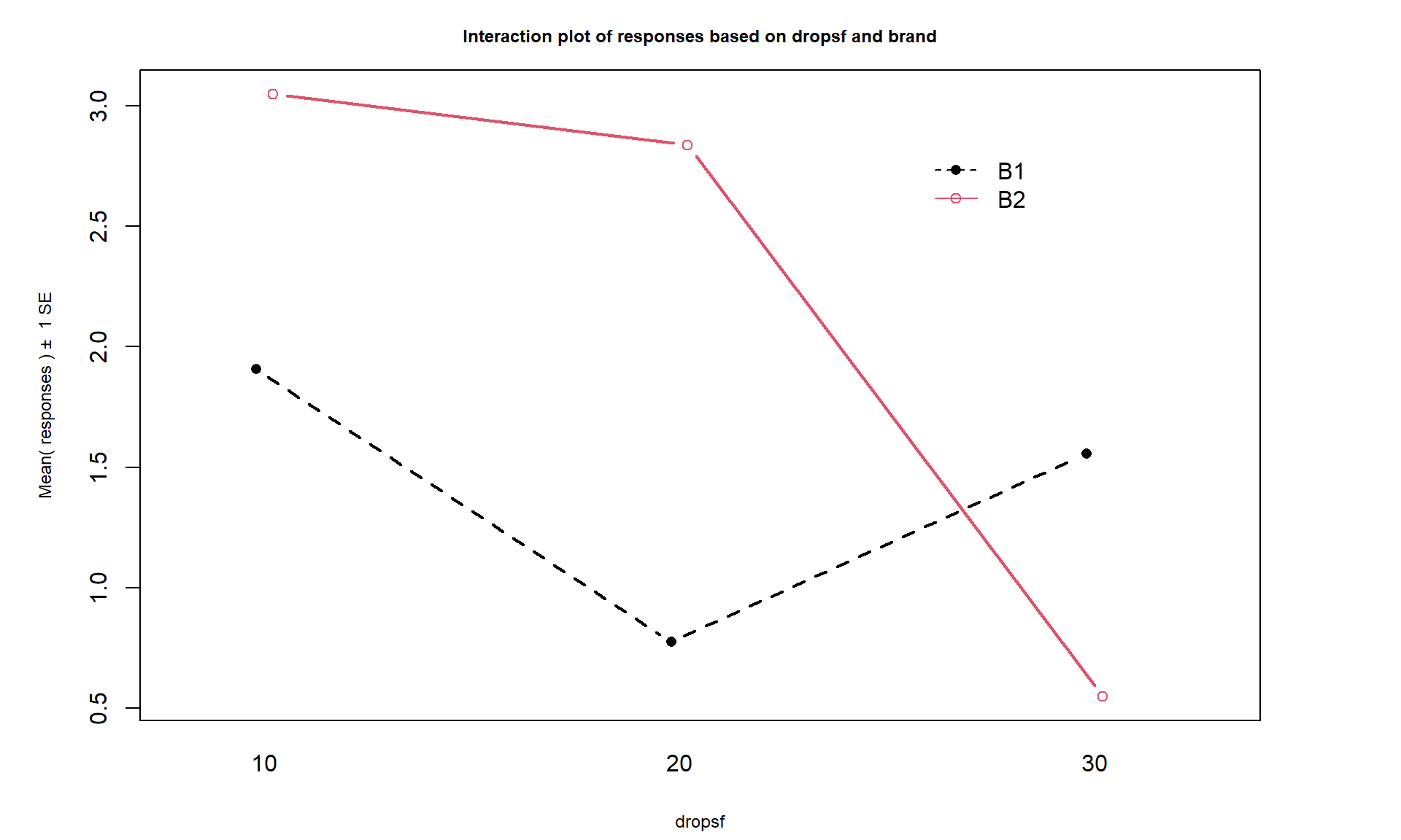
intplot(responses ~ brand * dropsf, data = ptR, lwd = 2)

The next step would be to assess evidence related to the null hypothesis of no interaction between Brand and Drops. A problem will arise in trying to form the ANOVA table as you would see this when you run the anova⁹⁴ function on the interaction model:

anova(lm(responses ~ dropsf * brand, data = ptR))

## Analysis of Variance Table
## Response: responses
##              Df  Sum Sq Mean Sq F value Pr(>F)
## dropsf        2 2.03872 1.01936               
## brand         1 0.80663 0.80663               
## dropsf:brand  2 2.48773 1.24386               
## Residuals     0 0.00000                       
## Warning message:
## In anova.lm(lm(responses ~ dropsf * brand, data = ptR)) :
##   ANOVA F-tests on an essentially perfect fit are unreliable

Warning messages in R output show up after you run functions that contain problems and are generally not a good thing, but can sometimes be ignored. In this case, the warning message is not needed – there are no \(F\)-statistics or p-values in the results so we know there are some issues with the results. The Residuals line is key here – Residuals with 0 df and sums of squares of 0. Without replication, there are no degrees of freedom left to estimate the residual error. My first statistics professor, Dr. Gordon Bril at Luther College, used to refer to this as “shooting your load” by fitting too many terms in the model given the number of observations available. Maybe this is a bit graphic but hopefully will help you remember the need for replication if you want to test for interactions – it did for me. Without replication of observations, we run out of information to test all the desired model components.

So what can we do if we can’t afford replication but want to study two variables in the same study? We can assume that the interaction does not exist and use those degrees of freedom and variability as the error variability. When we drop the interaction from Two-Way models, the interaction variability is added into the \(\text{SS}_E\) so we assume that the interaction variability is really just “noise”, which may not actually be true. We are not able to test for an interaction so must rely on the interaction plot to assess whether an interaction might be present. Figure 4.20 suggests there might be an interaction in these data (the two brands’ lines suggesting non-parallel lines). So in this case, assuming no interaction is present is hard to justify. But if we proceed under this dangerous and untestable assumption, tests for the main effects can be developed.

norep1 <- lm(responses ~ dropsf + brand, data = ptR)
Anova(norep1)

## Anova Table (Type II tests)
## 
## Response: responses
##            Sum Sq Df F value Pr(>F)
## dropsf    2.03872  2  0.8195 0.5496
## brand     0.80663  1  0.6485 0.5052
## Residuals 2.48773  2

In the additive model, the last row of the ANOVA table that is called the Residuals row is really the interaction row from the interaction model ANOVA table. Neither main effect had a small p-value (Drops: \(F(2,2) = 0.82, \text{ p-value} = 0.55\) and Brand: \(F(1,2) = 0.65, \text{ p-value} = 0.51\)) in the additive model. To get small p-values with the small sample sizes that unreplicated designs would generate, the differences would need to be very large because the residual degrees of freedom have become very small. The term-plots in Figure 4.22 show that the differences among the levels are small relative to the residual variability as seen in the error bars around each point estimate.

plot(allEffects(norep1))

Figure 4.22: Term-plots for the additive model in paper towel data set with no replication.

In the extreme unreplicated situation it is possible to estimate all model coefficients in the interaction model but we can’t do inferences for those estimates since there is no residual variability. Another issue in really any model with categorical predictors but especially noticeable in the Two-Way ANOVA situation is estimability issues. Instead of having issues with running out of degrees of freedom for tests we can run into situations where we do not have information to estimate some of the model coefficients. This happens any time you fail to have observations at either a level of a main effect or at a combination of levels in an interaction model.

To illustrate estimability issues, we will revisit the overtake data. Each of the seven levels of outfits was made up of a combination of different characteristics of the outfits, such as which helmet and pants were chosen, whether reflective leg clips were worn or not, etc. To see all these additional variables, we will introduce a new plot that will feature more prominently in Chapter 5 that allows us to explore relationships among a suite of categorical variables – the tableplot from the tabplot⁹⁵ package (Tennekes and de Jonge 2019). If this does not work, please contact your instructor or me for more information on possibly additional steps to get it working. The tabplot package allows us to sort the variables based on a single variable (think about how you might sort a spreadsheet based on one column and look at the results in other columns). The tableplot function displays bars for each response in a row⁹⁶ based on the category of responses or as a bar with the height corresponding the value of quantitative variables⁹⁷. It also plots a red cell if the observations were missing for a categorical variable and in grey for missing values on quantitative variables. The plot can be obtained simply as tableplot(DATASETNAME) which will sort the data set based on the first variable. To use our previous work with the sorted levels of Condition2, the code dd[,-1] is used to specify the data set without Condition and then sort = Condition2 is used to sort based on the Condition2 variable. The pals = list("BrBG") option specifies a color palette for the plot that is color-blind friendly from the RColorBrewer package (Neuwirth 2022).

dd <- read_csv("http://www.math.montana.edu/courses/s217/documents/Walker2014_mod.csv")

dd <- dd %>% mutate(Condition = factor(Condition),
                    Condition2 = reorder(Condition, Distance, FUN = mean),
                    Shirt = factor(Shirt),
                    Helmet = factor(Helmet),
                    Pants = factor(Pants),
                    Gloves = factor(Gloves),
                    ReflectClips = factor(ReflectClips),
                    Backpack = factor(Backpack)
                    )

library(remotes); 
remotes::install_github("mtennekes/tabplot") # Only do this once on your computer

library(tabplot)
library(RColorBrewer)
# Options (sometimes) needed to prevent errors on PC
# options(ffbatchbytes = 1024^2 * 128); options(ffmaxbytes = 1024^2 * 128 * 32) 
tableplot(dd[,-1], sort = Condition2, pals = list("BrBG"), sample = F, 
          colorNA_num = "pink", numMode = "MB-ML")

Figure 4.23: Tableplot of the full overtake data set sorted by outfit worn (Condition2).

In the tableplot in Figure 4.23, we can now explore the six variables created related to aspects of each outfit. For example, the commuter helmet (darkest shade in Helmet column) was worn with all outfits except for the racer and casual. So maybe we would like to explore differences in overtake distances based on the type of helmet worn. Similarly, it might be nice to explore whether wearing reflective pant clips is useful and maybe there is an interaction between helmet type and leg clips on impacts on overtake distance (should we wear both or just one, for example). So instead of using the seven level Condition2 in the model to assess differences based on all combinations of these outfits delineated in the other variables, we can try to fit a model with Helmet and ReflectClips and their interaction for overtake distances:

overtake_int <- lm(Distance ~ Helmet * ReflectClips, data = dd)
summary(overtake_int)

## 
## Call:
## lm(formula = Distance ~ Helmet * ReflectClips, data = dd)
## 
## Residuals:
##      Min       1Q   Median       3Q      Max 
## -115.111  -17.756   -0.611   16.889  156.889 
## 
## Coefficients: (3 not defined because of singularities)
##                            Estimate Std. Error t value Pr(>|t|)
## (Intercept)                117.1106     0.4710 248.641   <2e-16
## Helmethat                    0.5004     1.1738   0.426    0.670
## Helmetrace                  -0.3547     1.1308  -0.314    0.754
## ReflectClipsyes                  NA         NA      NA       NA
## Helmethat:ReflectClipsyes        NA         NA      NA       NA
## Helmetrace:ReflectClipsyes       NA         NA      NA       NA
## 
## Residual standard error: 30.01 on 5687 degrees of freedom
## Multiple R-squared:  5.877e-05,  Adjusted R-squared:  -0.0002929 
## F-statistic: 0.1671 on 2 and 5687 DF,  p-value: 0.8461

The full model summary shows some odd things. First there is a warning after Coefficients of (3 not defined because of singularities). And then in the coefficient table, there are NAs for everything in the rows for ReflectClipsyes and the two interaction components. When lm encounters models where the data measured are not sufficient to estimate the model, it essentially drops parts of the model that you were hoping to estimate and only estimates what it can. In this case, it just estimates coefficients for the intercept and two deviation coefficients for Helmet types; the other three coefficients (\(\gamma_2\) and the two \(\omega\)s) are not estimable. This reinforces the need to check coefficients in any model you are fitting. A tally of the counts of observations across the two explanatory variables helps to understand the situation and problem:

tally(Helmet ~ ReflectClips, data = dd)

##           ReflectClips
## Helmet       no  yes
##   commuter    0 4059
##   hat       779    0
##   race        0  852

There are three combinations that have \(n_{jk} = 0\) observations (for example for the commuter helmet, clips were always worn so no observations were made with this helmet without clips). So we have no hope of estimating a mean for the combinations with 0 observations and these are needed to consider interactions. If we revisit the tableplot, we can see how some of these needed combinations do not occur together. So this is an unbalanced design but also lacks necessary information to explore the potential research question of interest. In order to study just these two variables and their interaction, the researchers would have had to do rides with all six combinations of these variables. This could be quite informative because it could help someone tailor their outfit choice for optimal safety but also would have created many more than seven different outfit combinations to wear.

Hopefully by pushing the limits there are three conclusions available from this section. First, replication is important, both in being able to perform tests for interactions and for having enough power to detect differences for the main effects. Second, when dropping from the interaction model to additive model, the variability explained by the interaction term is pushed into the error term, whether replication is available or not. Third, we need to make sure we have observations at all combinations of variables if we want to be able to estimate models using them and their interaction.